Fat Chance and Probability HardvardX Course Notes
1. Basic Counting
Probabilities are always the count of some events divided by the count of another set of events.
There are $n$ numbers between the numbers $1$ and $n$, including $n$ and $1$.
The total number of numbers between $k$ and $n$, where $n>k$, is $n-k+1$, including $k$ and $n$.
If you have a m-digit number in a numbers system with base $b$ then there are $b^m$ different numbers you could have, including $0$ and the last number is $(b^m)-1$
- E.g. in a base 10 ($b=10$) system a 32 ($m=32$) digit number means there are $10^{32}$ distinct numbers
- E.g. in a binary ($b=2$) system a 8 ($m=8$) digit number means there are $2^8=256$ distinct numbers where $0$ is the first and the last number is $11111111=255$
The Subtraction Principle: The number of objects in a collection that satisfy some condition is equal to the total number of objects in the collection minus
the number in that collection that don't satisfy the condition. It's sometimes easier to count the objects that don't satisfy the condition,
Multiplication principle
The number of ways of making a sequence of independent choices is just the product of the number of choices at each step.
In this context independent means that the first choice you make doesn't affect the number of choices at the second step and so on.
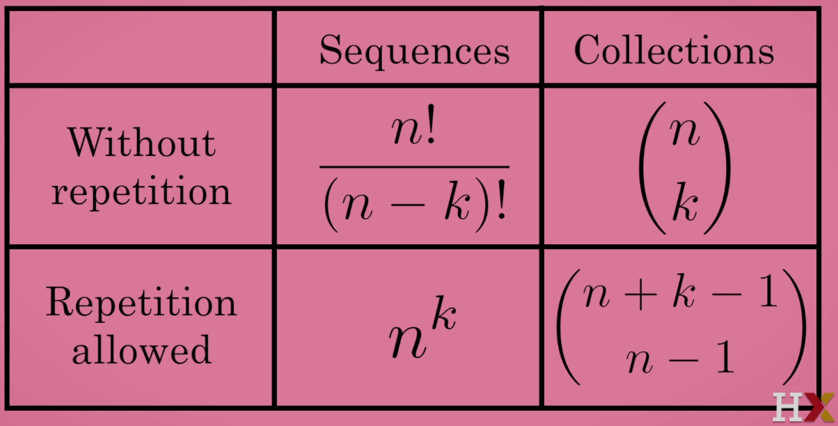
The number of possibilities (sequences) of $k$ object chosen from a collection of $n$ objects is $n^k$
- E.g. imagine you have 4 buckets ($k=4$) where each bucket represents a game of soccer between two teams in each game either Team A wins, Team B wins or A and B Tie so in each bucket has 3 balls each represents the result of the game ($n=3$)
the number of results that can occur is $3^4=81$
- E.g. imagine you have 2 buckets ($k=2$), each buckets have 26 different letters ($n=26$) how many two letter words can you form (you take one letter from the fist bucket and another from the second bucket). Answer: $26^2$
The number of sequences of $k$ objects (seats) chosen without repetition from a collection of $n$ objects (options). Number of sequences of $k$ objects chosen without repetition from a pool of $n$ objects.
- E.g. imagine we have 4 different students Student A, B, C and D ($n=4$) and we have to select president (P) and vice-president (VP) of the class ($k=2$) how many ways there are to assign these charges. Answer: $4 \cdot (4-2+1)=4 \cdot 3=12$
The number of sequences of $k$ objects chosen without repetition from a collection of $n$ objects can be written more compactly as $n!/(n-k)!$.
2. Advance Counting
Sequence Objects in a sequence are ordered we know what element is the first element in the sequence, and what's second, and what's third, and what's fourth, etc.
Collection Objects in a collection are not ordered, it doesn't matter in which order we select elements from another collection
The number of ways of choosing a collections of $k$ objects without repetition from a set of $n$ objects is $N=n!/((n-k)! \cdot k!)$ this is called the binomial coefficient $(n, k) = n!/((n-k)! k!)$ where $ 1 \lt k \lt n $
- The number of hands ($N$) in a 5 card poker game ($k = 5$) using only one deck of 52 cards ($n = 52$), since only one deck is being used this also implies no repetition is $(52, 5) = 52!/((52-5)! \cdot 5!)$
Binomial coefficient properties
- It is a whole number
- $(n,k) = (n, n-k)$
- $(n,k) = (n-1, k) + (n-1, k-1)$
The Multinomial coefficient (multinomials) is the generalization of the binomial coefficient.
Suppose we have a pool of $n$ objects and we want to divide them up into $k$ collections of sizes $a1$, $a2$, $a3$, ..., $ak$ where $n = a1 + a2 + a3 + ... + ak$
This is given by $(n ; a1, a2, ..., ak) = n!/(a1! \cdot a2! \cdots ak!)$
The number of collections of $k$ objects chosen from a pool of $n$ objects with repetition allowed is $(n+k-1 , k) = (n+k-1 , n-1)$
3. Basic Probability
- The probability of a favorable outcome = Number of favorable outcomes/Number of all possible outcomes
Probability and Statistics for Business and Data Science
Data
- Data The collected observations we have about something that helps us understand things as they are. Types of data:
- Continuous: You have a continuous range where you can keep getting finer and finer
- e.x. What is the stock price of Tesla? you can get the price right now and that is a data point, then you can get it one minute later or 30 seconds later or 1 seconds later and so on
- Categorical helps categorize or group objects. You have a categorical data point, each of those are categories and there is nothing in between them
- e.x. What car has the best repair history? WV, Honda, Nissan, etc each of the brands is a categorical point
Visualizations and analytical techniques only work on certain types of data (some only work on continuous, some only in in categorical data)
We use data to try to see if there is a relationship between two events and try to predict future behavior
Levels of measurement:
- Nominal Predetermined categories that cannot be sorted. E.x. animal classification: mammal, fish, reptile ; car brand: WV, Chevy, Toyota
- Ordinal Can be sorted but lacks numerical scale but can have certain order or categories for example a Never-Rarely-Sometimes-Always survey
- Ordinal Provides a scale but has no reference or zero point. e.x. Temperature or thermometer that starts at 30C
- Ratio Provides a scale and has a reference or zero point, no negative values. e.x. Age, Weight, Salary
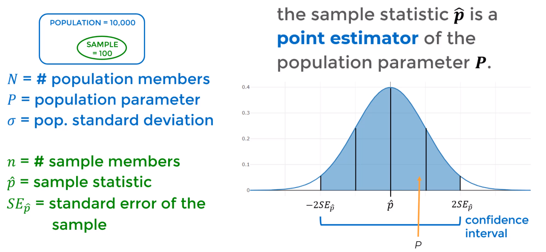
The Population refers to every member of a group we want to study (this can be defined differently depending on the context. e.x. every person in the world or everyone in a particular city) while a Sample is subset or small set of members from the population that time and resources allow you to measure
Measurements of central tendency
Measurements of central tendency are measurements (numbers) that gives us the Average of or data, this means the center of the data or general location of the data
- Describe location of the data (where it is mostly located) but don't describe the shape of the data (how spread the data is)
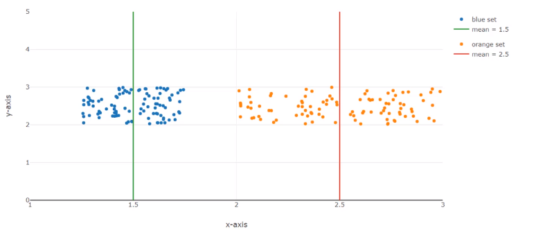
Mean/Sample Mean: calculated average. Sum all the elements and dive by the number of elements. $\boxed{\bar x = \dfrac{\sum_{i=1}^n x_i}{n}}$
- It can be influenced by outliners (values that are very different from the most common ones)
Median: Middle value in a data set sorted.
- To calculate you always need to sort first then:
- For Odd number of values: Take the element given by the index =
floor(len(data)/2)
- For Even number of values: Get the two values in the middle and get average ->
(floor(len(data)/2) + floor(len(data)/2)-1)/2
Mode: The most common value in a data set, so just get the most repeated value
Measurements of Dispersion
The Measurements of Dispersion tell us how disperse the data is or how spread out the data is
To know how far from the average did an individual value stray we sue Measure of Dispersion
Range: Difference between the max and minimum value $$R = max - min$$
Variance: It tells you how far away are all your points from the mean or center but returns the units squared. Calculated as the sum of square distances from each point to the mean
- Sample variance: $S^2 = \dfrac{\sum_{i=1}^m (x_i-\bar x)^2}{n-1}$
- Population variance: $\sigma^2 = \dfrac{\sum_{i=1}^m (X_i-\mu)^2}{N}$
Standard Deviation: Allow you to describe values that lie within one, two, three, etc standard deviations of the mean. Calculated as the square root of the variance to get the same units as the sample
- Sample Standard Deviation: $S = \sqrt{^2} =\sqrt{\dfrac{\sum_{i=1}^m (x_i-\bar x)^2}{n-1}} $
- Population Standard Deviation: $\sigma = \sqrt{\sigma^2} = \sqrt{\dfrac{\sum_{i=1}^m (X_i-\mu)^2}{N}}$
In general the population Standard Deviation and the sample Standard Deviation tend to be similar
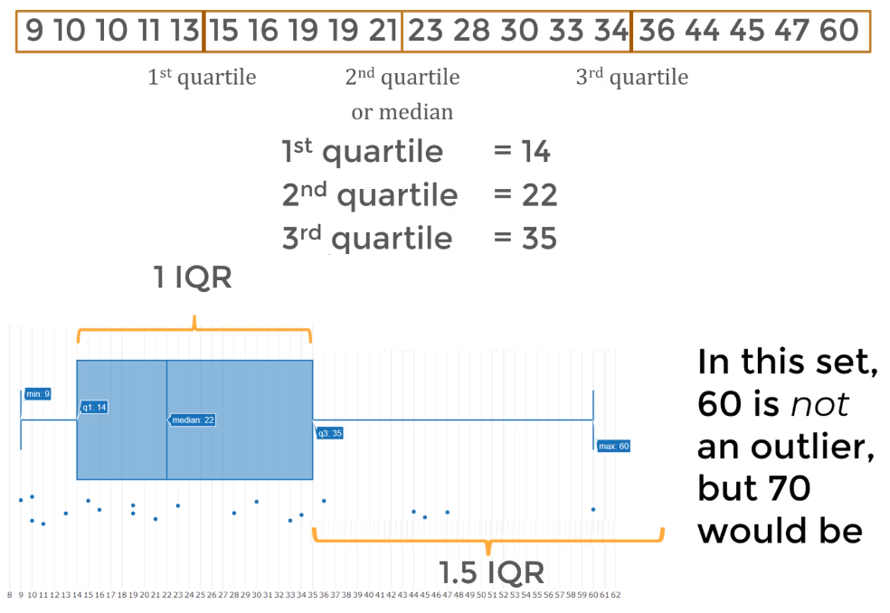
Quartiles & IQR (Interquartile Range)
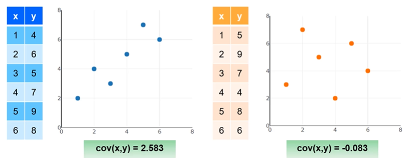
Correlation, Covariance & Pearson Coefficient
Bivariate Data refers to comparing two variables (like in a math function) while if you are dealing with a single array or set of data, those are referred as univariate data sets
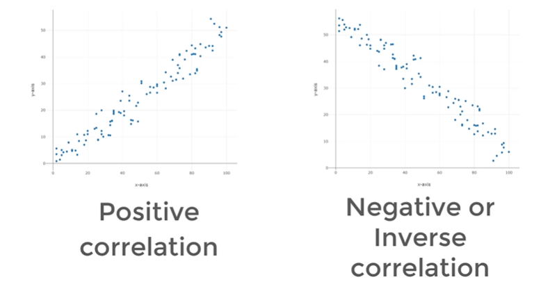
Scatter plots are a graphical way to know if there is a correlation
The correlation between two variables refers to the relationship between two sets of variable values used to describe or predict information. If variables have a correlation it means they are in sync with each other
- Positive: as you increase one variable the other increases
- Negative: as you increase one variable the other decreases
Correlation does not imply causality (it can, but not always. In other words It can't prove it definitely)
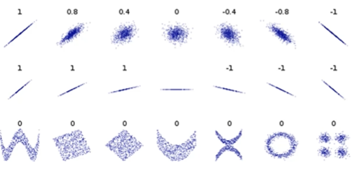
- The Pearson Correlation Coefficient is the most common way to describe correlation between two variables, which normalizes covariance to be between $[-1,1]$
- $+1$ Total positive linear correlation. if one values goes up or down the other does the same in perfect sync
- $0$ No linear correlation
- $-1$ Total negative linear correlation. if one values goes up the other goes down (doing the opposite)
$$\rho_{x,y} = \dfrac{cov(x,y)}{\sigma_x \sigma_y} = \dfrac{\sum_{i=1}^N (x_i-\bar x)(y_i-\bar y)}{\sqrt{\sum_{i=1}^N (x_i-\bar x)^2} \sqrt{\sum_{i=1}^N(y_i-\bar y)^2}}$$
Probability
- Probability is a value between 0 and 1 that a certain event will occur after we perform a trial (test). It is sometimes expressed as a percentage which results from multiplying by 100. Each trial is usually called experiment and each different and exclusive outcome is a simple event while the sample space is the sum of every possible simple event
- Examples:
- The probability that a coin comes up as heads (event: result is heads) after flipping (trial: flipping coin) is 0.5 or 50% the simple events are two: $E_1=Heads$ and $E_2=Tails$ so the sample space is $S=\{E_1, E_2\}$
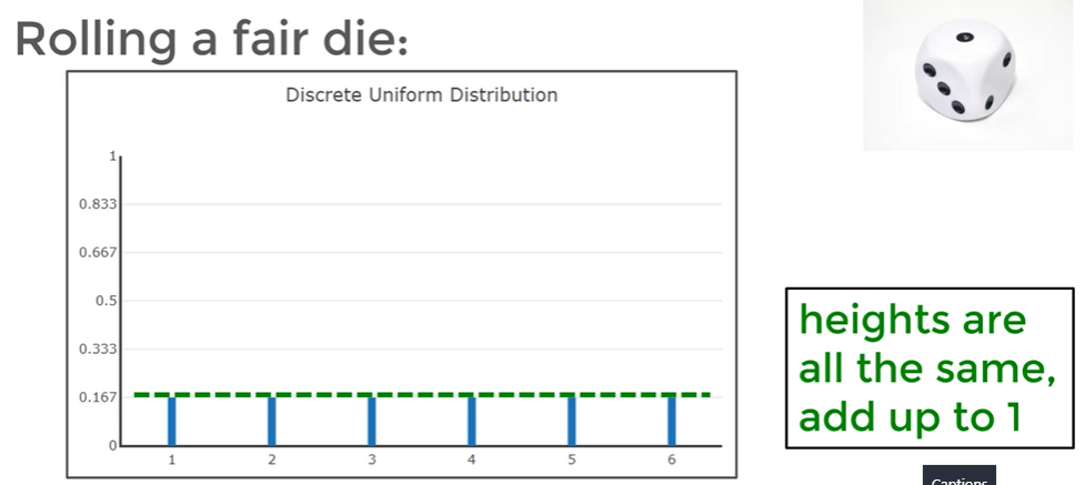
- The probability that a dice comes up as 6 (event) after rolling it (trial) is 1/6, the simple events are six: $E_1=1$, $E_2=2$, $E_3=3$, $E_4=4$, $E_5=5$ and $E_6=6$ so the sample space is $S=\{E_1, E_2, E_3, E_4, E_5, E_6\}$
$$P(Event) = P_{Value}$$
Trials are independent in other words they have no memory so you can't think of a series of independent events to affect each other
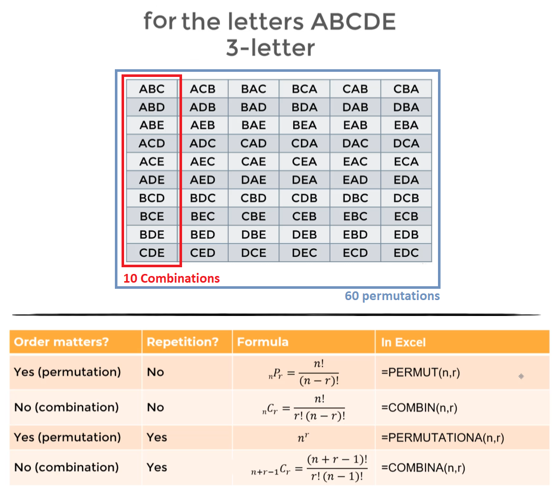
A Permutation of a set of objects is an arrangement of the objects in a certain order
- The possible permutations tell us all the possible ways we can arrange/accommodate a set of objects
- Permutation no repetitions: The number of permutations of a set of $n$ objects taken $r$ at a time is $P_{(n,r)}=\dfrac{n!}{(n-r)!}$
- Example: How many different 4-character passwords are if we can only use lowercase letters and numbers from 0-9 consider we cannot repeat characters (no repetitions) $P_{(36, 4)}=\dfrac{36!}{(36-32)!}=\dfrac{36!}{32!}=1413720$
- Permutation with repetitions: The number of permutations of a set of $n$ objects taken $r$ at a time allowing repetition is $P_{(n,r)}=n^r$
- Example: How many different 4-character license plates can you make using numbers 0-9 allowing repetition (with repetitions) $P_{(10, 4)}=10^4$
A Combination is an unordered arrangement of objects, represent a combination of unique elements
- Combination no repetitions: of a set of $n$ objects taken $r$ at a time is $C_{(n,r)}=\dfrac{n!}{r!(n-r)!}$
- Example: How many different class teams of 3 people can you create if you have only 5 people in class $C_{(5,3)}=\dfrac{5!}{3!(5-3)!}=10$
- Combination with repetitions: of a set of $n$ objects taken $r$ at a time allowing repetition is $C_{(n,r)}=\dfrac{(n+r-1)!}{r!(n-1)!}$
- Example: In a pizzeria you have 10 ingredients for a pizza a customer can chose 4 ingredients and repetition of ingredients is allowed how many different pizzas can a customer select? $C_{(10,4)}=\dfrac{(10+4-1)!}{4!(10-1)!}=715$
An Independent series of events occur when the outcome of one event has no effect on the outcome of another. The probability of seeing two or more independent events is $P(E_1,E_2,\ldots,E_n) = P(E_1) \cdot P(E_2) \cdots P(E_n)$
A Dependent ever occurs when the outcome of the first event does affect the probability of a second event. The probability of a current event 2 to occur $E_2$ given that a previous event 1 $E_1$ occurred $P(E_2 | E_1)$
The probability that two events occur consecutively is given by the intersection $P(E_2 \cap E_1) = P(E_1) \cdot P(E_2 | E_1)$
Conditional probability is the idea that we want to know the probability of current event $E_2$ given that a previous event $E_1$ has occurred. $P(E_2|E_1)=P(E_{current}| E_{previous})$
$$P(E_2|E_1) = \dfrac{P(E_2 \cap E_1)}{P(E_1)} = P(E_{current}|E_{previous}) = \dfrac{P(E_{previous} \cap E_{current})}{P(E_{previous})}$$
The probability of current event given a previous event occurred is equal to the probability of both occur divided by the probability of that the previous event occurs
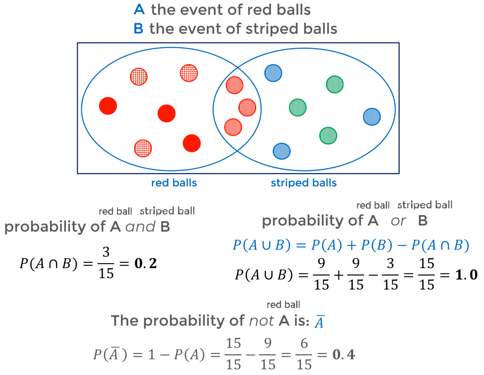
The Complement (not $A$ -> $\bar A$) of an event considers everything outside of the event. In other words where the event does not occur. $P(\bar A) = 1-P(A)$
In probability an Intersection ($A$ and $B$ -> $A \cap B$) describes the sample space where two events both occur $A and $B$. $P(A \cap B)$
- The Multiplication Rule: $P(A \cap B) = P(A) \cdot P(B | A)$. Probability of $A$ and $B$ is given by the probability of $A$ multiplied by the probability that $B$ occurs given $A$ has occurred. $P(A \cap B \cap C \cdots \cap Z) = P(A) \cdot P(B|A) \cdot P(C|AB) \cdot P(D|ABC) \cdots P(Z|ABCD \cdots Y)$
In probability unions ($A$ or $B$ -> $A \cup B$) considers if one event or the other occurs (either event occurs).
- The Addition Rule: $P(A \cup B) = P(A) + P(B) - P(A \cap B)$
- The Addition Rule for Mutually Exclusive Events (For two events that cannot both happen or be true at the same time): $P(A \cup B) = P(A) + P(B)$
- Bayes Theorem results from combining the multiplication rules ($P(A \cap B)$ and $P(B \cap A)$) it is used to determine the probability of a parameter given a certain event $P(A|B)=\dfrac{P(B|A)P(A)}{P(B)}$
Distributions
- A distribution describes all of the probable outcomes of a variable
Discrete probability distributions
- In a discrete distribution/probability mass functions the sum of all individual probabilities must equal 1. In a discrete refers to de ideas that the distribution only has certain probable outcomes like 1,2,3, etc but not values in between like 1.5 or 2.75
- The Uniform Distribution has discrete equally probable outcomes, so the outcomes are evenly distributed across the sample space
Binomial Distribution
The Binary/Binomial Distribution has two discreate mutually exclusive outcomes ( binomial outcomes) like: heads/tails, on/off, pass/fail. etc
A Bernoulli Trial is a random experiments with two possible outcomes: Success | Failure. For a series of $n$ trials
- The probability of success $p$ is constant
- Trials are independent of one another (one trial does not affect the following ones)
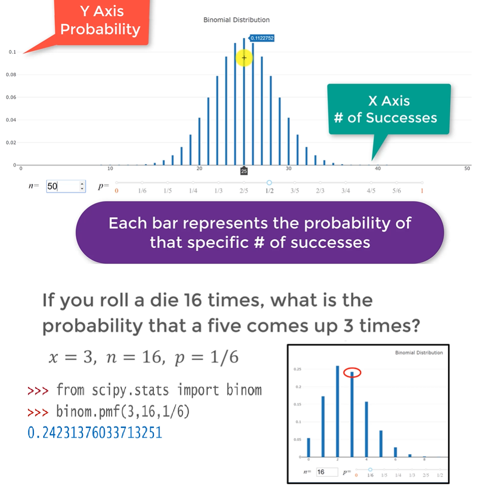
The Binomial Probability Mass Function Gives the probability of observing $x$ number of successes after doing $n$ number of trials. The probability of success on a single trial is denoted by $p$ and it is the same (fixed) for all trials
- $x$: number of successes
- $n$: number of trials
- $p$: probability of success on single trial
$$\binom{n}{x} = \dfrac{n!}{x!(n-x)!} \hphantom{\text{space}} P(x:n,p) = \binom{n}{x}p^x(1-p)^{(n-x)} = \dfrac{n!}{x!(n-x)!}p^x(1-p)^{(n-x)}$$
Poisson Distribution
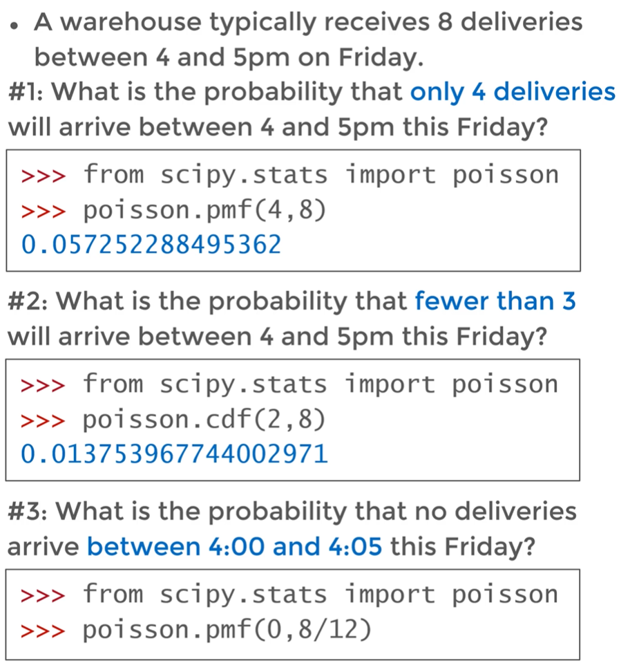
- Poisson Distribution considers the number of successes per continuous unit (usually time) for a certain number of units. Number of success per second for a certain amount of time for example an hour
- $x$: number of occurrences
- $P(x)$: probability of that many occurrences
- $\mu=\lambda$: Number of occurrences per interval, average of occurrences per unit e.x. 10 cars per hour, 15 semaphores per kilometer, etc
$$\mu = \lambda = \dfrac{\text{# occurrences}}{\text{interval}} \hphantom{\text{space}} P(x) = \dfrac{\lambda^x e^{-\lambda}}{x!}$$
The highest probability of occurrence is centered around the average $\lambda$/$\mu$
- Cumulative mass function used to get the probability to see less or equal to certain number of occurrences $N$ in the Poisson Distribution e.x. the probability of seeing less than 4 ($N=3$) occurrences or the probability of seeing less or equal than 4 ($N=4$) occurrences
$$ P(X, x < N) = \sum_{i=0}^{N-1} \dfrac{\lambda^i e^{-\lambda}}{i!} $$
$$ P(X, x \le N) = \sum_{i=0}^{N} \dfrac{\lambda^i e^{-\lambda}}{i!} $$
- The probability of seeing at least one event $P(X, x \ge 1) = 1 - \dfrac{\lambda^0 e^{-\lambda}}{0!} = 1-e^{-\lambda}$
The sum all possibilities should be equal to one
- The Poisson distribution applies only when the probability of success in a certain interval ($\lambda$) is proportional to the entire length of the interval, so it assumes that if you know $\lambda$ for a interval of one hour then $\lambda$ for an interval of one minutes is proportional $\lambda_{min} = \lambda_{hour}/60$
Poisson distribution is essentially looking for a successful occurrences per some continuous unit (within a given interval) like unit of time or unit of distance
Continuous probability distributions
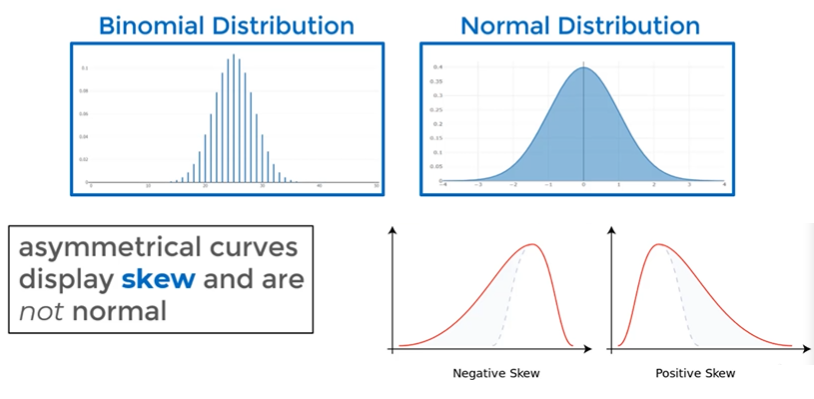
Normal Distribution
Normal Distributions are also called Gaussian Distributions or Bell curve
Many real life data points like (People's height|weights, blood pressure, test scores, measurement of errors, noise, etc) follow Normal Distributions
Data sources that follow the normal distributions tend to be around a central value with no bias to left or right, they are symmetrical
The probability of any specific outcome is zero we can only find probability over an specified interval or range of outcomes
- The Standard Normal Distribution is a specific variant of the normal distribution where:
- its mean is zero ($\mu=0$) and standard deviation is 1 $\sigma = 1$
- 68.27% of all possible values are going to fall within one standard deviation
- 95.45% of all possible values are going to fall within two standard deviations
- 99.73% of all possible values are going to fall within three standard deviations
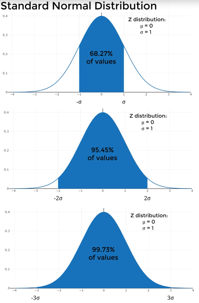
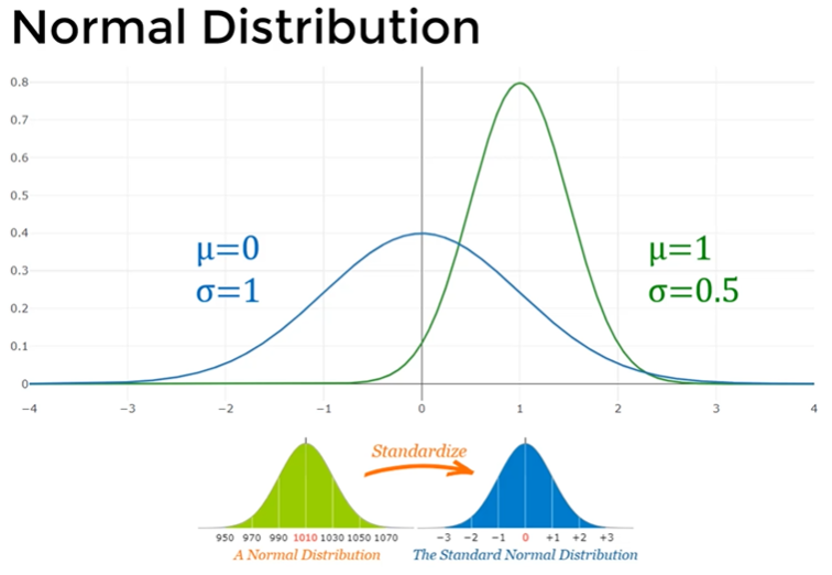
The Normal Distribution curves follow the same symmetry about the mean and 99.73% of all values fall within three standard deviations but the mean doesn't have to be zero ($\mu \ne 0$) and standard deviation doesn't have to be 1 $\sigma \ne 1
If we determine a data set approximates a normal distribution we can make powerful inferences about it once we know its mean and standard deviation
We can transform any normal distribution and standardize it to a standard normal distribution by using Z score
A percentile is a way of saying what percentage of values falls below this value, what percentage of the values fall in a value less than this ones
- e.x. student scores a 9 and this score is in the 90 percentile we know 90& of all other students scored less than 9
Normal distribution function: $f(x) = \dfrac{1}{\sqrt{2\pi\sigma^2}}e^{-\dfrac{(x-\mu)^2}{2\sigma^2}}$
- $\mu$: mean
- $\sigma$: standard deviation
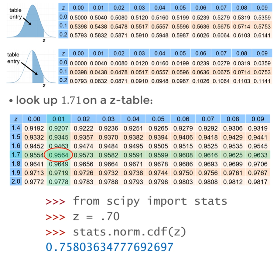
- To gain insight about a specific value of $x$ we standardize by calculating a z-score $z=\dfrac{x-\mu}{\sigma}$ then use a z-table that maps a z-score particular value to the area under a normal distribution curve
Statistics
Statistics is the application of what we know to what we want to know. We apply statistical inferences to a sample to try to describe a population and usually a reasonable size (>32) random sample will almost always reflect the population
a parameter is a characteristic of a population
a statistic is a characteristic of a sample
a variable is a characteristic that describes a member of the sample and can be discreate (e.x. birthplace gender) or continuous (e.x. salary, age)
Bias:
- Selection bias: select members who are inclined or can participate (e.x. select only people willing to answer a poll)
- Survivorship bias: if a population increases it may be due to lesser members leaving, dying or being expelled or reallocated
Types of Sampling:
- Random: Randomly select
- $+$: Every member of the population has equal chance of being selected
- $–$: since samples are much smaller than population there is high chance the entire demographic might be missed
- Stratified Random Sampling: Divide into segments based on characteristic and take a random sample from each group, the size of the sample is based on the size of the group relative to the population. You need to make sure members cannot below two to groups at once
- $+$: Compensates by trying to ensure groups within a population are adequately represented
- Clustering break population intro groups and sample only a random selection of groups (clusters)
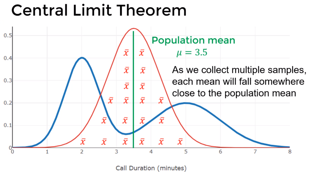
Central limit Theorem (CLT) the mean values from a group of samples will be normally distributed about the population mean even if the population itself is not normally distributed
- Which means 95% of all sample means should fall within $2\sigma$ of the population mean
- Sample means follow a normal distribution about the population mean
- If you take many samples of a population then you get the mean of all those groups of samples, those means will be normally distributed around the mean of the entire population even if the population itself is not normally distributed
- Standard Error of the mean: while the population standard deviation describes how wide individual values stray from the population mean the standard error of the mean describes how far a sample mean stray from the population mean $SE_{\bar x} = \dfrac{\sigma}{\sqrt{n}}$
- It shows you the relationship between the sample mean and the population mean
- We can say with a 95% confidence level that a population parameter () lies within a confidence interval of plus-or-minus two standard error of the sample statistic
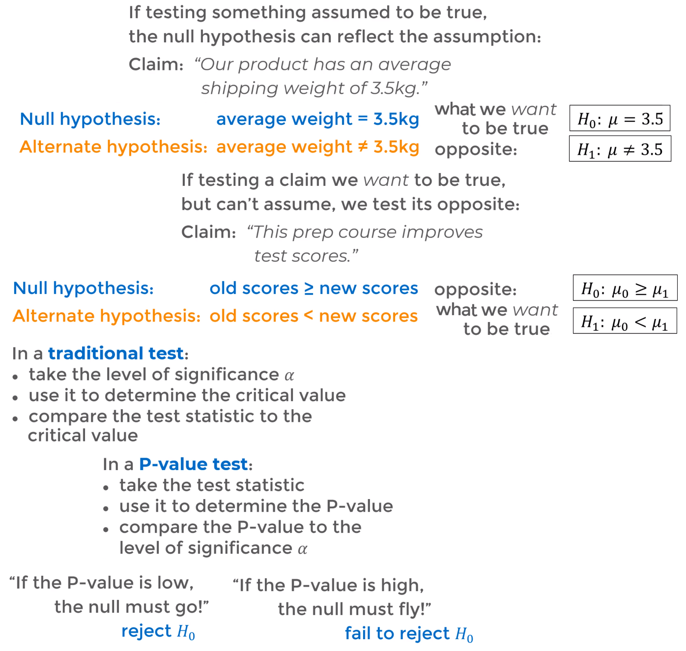
- Hypothesis Testing is the application of statistical methods to real-world questions
- State Null Hypothesis: We start with an assumptions, the null hypothesis ($H_0 =H_{null}$) and alternate hypothesis ($H_1 =H_{alt}$)
- The null hypothesis should contain an equality, this means it can be: $=$, $\le$, $\ge$
- The alternate hypothesis should not have equality, this means it can be: $\ne$, $<$, $>$
- Significance & Test type: Set level of significances and based on hypothesis determine type of test
- level of significance $\alpha$ usually is $\alpha = 0.05$
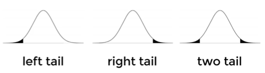
- Determine rejection area critical values/z-scores:
- left-tail: $(H_1 = H_{alt}) < (H_{null} = H_0)$
- right-tail: $(H_1 = H_{alt}) > (H_{null} = H_0)$
- two-tails: $(H_1 = H_{alt}) \ne (H_{null} = H_0)$
- Calculate Z: We run an experiment to test this null hypothesis and record the result. Calculate $Z$ (test statistic)
- Tests of Mean are used when we look to find an average or specific value in a population (deal with means/average of the population)
- $Z= \frac{\bar x - \mu}{\sigma/\sqrt{n}}$
- $\bar x$: sample mean
- $\mu$: population mean
- $\sigma$: population standard deviation (assumes we know this)
- $n$ number of samples
- Tests of proportion are used when we look for a range of certain percent of the population for example when we say certain percent or more / certain percent or less (deal with percentage of the population)
- $Z= \frac{\hat p - p}{\sqrt{(p \cdot (1-p))/n}}$
- $n$ number of samples
- $\hat p$ Actual sample proportion (usually a percentage 58%=0.58)
- $p$ The proportion we are looking for (usually a percentage 50%=0.5)
- Table lookup: get value from table
- For z-value look up, you use $\alpha$ to get a z-value that will be compared against the $Z$ (calculated in prev step)
- For p-value look up, you use $Z$ (calculated in prev step) and get a p-value $P$ that will be compared against $\alpha$
- Evaluation to Reject/Fail to Reject: Based on results from experiment (calculations) we reject or fail to reject/no-reject the null hypothesis
- Fail to reject null hypothesis, $Z$ is outside rejection area
- $Z$(test statistic) is greater than found $z$ value so $Z > z$ is true for left-tail and $Z < z$ is true for right-tail
- if $P$ is greater than level of significance so $P > \alpha$ is true for left-tail and $P < \alpha$ is true for right-tail
- Reject null hypothesis, $Z$ is inside rejection area
- $Z$(test statistic) is greater than found $z$ value so $Z > z$ is true for right tail and $Z < z$ is true for left-tail
- if $P$ is greater than level of significance so $P>\alpha$ is true for right tail and $P < \alpha$ is true for left-tail
- If null hypothesis rejected then the data supports another mutually exclusive alternate hypothesis but we never prove the hypothesis
- If data fails to support the null hypothesis (we reject it) only then we can look for alternative hypothesis
Sample size matters for Hypothesis Testing. As sample size increases, the Standard Error of the Mean:
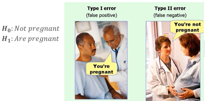
- Type 1 Error/False Positive reject a null hypothesis that should have been supported
- Examples: House fire alarm says there is a fire, you reject it (ignore it) because you don't see or smell any smoke in your room then realize the kitchen in another room was actually on fire
- Type 2 Error/False Negative accept (fail to reject) a null hypothesis that should have been rejected
- Examples: House fire alarm says there is a fire, you accept without checking all the rooms and call the fire department they arrive and realize there is no fire and your alarm is failing
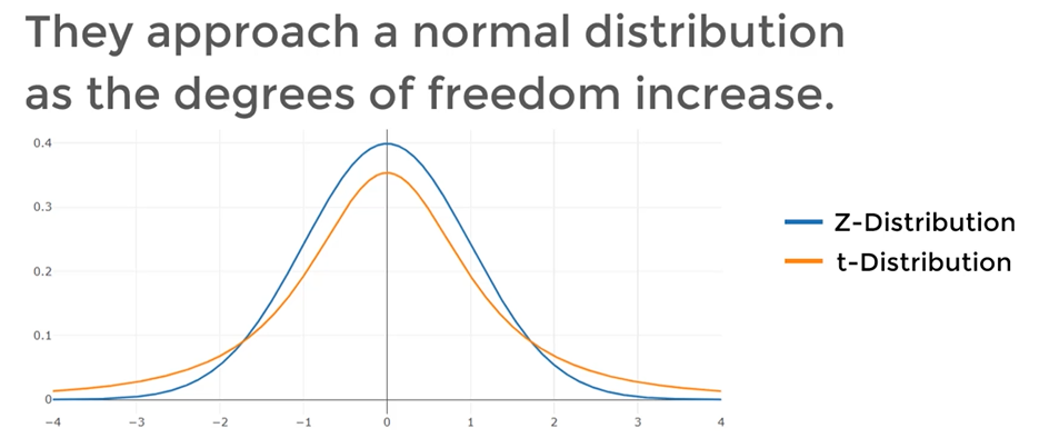
- Using a t-table a t-test determines if there is a significance difference between two sets of data
- One-sample t-test test that the population mean is equal to a value $\mu$ based on a sample mean $\bar x$
- formula: $t = \dfrac{\bar x -\mu}{s/\sqrt{n}}$
- $\bar x$ sample mean
- $\mu$ population mean
- $s$ sample standard error
- $n$ sample size
- Compare t-score: $t \gtrless t_{n-1,\alpha}$
- $t$ t-statistic
- $t_{n-1,\alpha}$ t-critical threshold
- $n-1$ degrees of freedom
- $\alpha$ significance level
- e.x. want to check if a sample of students scores have the same mean test scores as as population of students
- Independent two-sample t-test: test that two sample means $\bar x_1$ and $\bar x_2$ are equal. Calculate the ratio of signal-to-noise
- formula for equal or unequal samples size with unequal variance $t=\dfrac{\text{signal}}{\text{noise}}=\dfrac{\text{diff in means}}{\text{sample variability}} = \dfrac{\bar x_1 - \bar x_2}{\sqrt{s_1^2/n_1 + s_2^2/n_2}}$
- $\bar x_1, \bar x_2$ sample means
- $s_1, s_2$ sample variances
- $n_1, n_2$ sample sizes
- Compare t-score: $t \gtrless t_{df,\alpha}$
- $t$ t-statistic
- $t_{df,\alpha}$ t-critical threshold
- $df$ degrees of freedom $df=\dfrac{(s_1^2/n_1 + s_2^2/n2)^2}{\dfrac{1}{n_1-1}(s_1^2/n_1)^2 +\dfrac{1}{n_2-1}(s_2^2/n_2)^2} \approxeq n_1 + n_2 - 2$
- $\alpha$ significance level
- e.x. want to check if the mean test scores of two separate sample of students have a significant difference
- Dependent paired-sample t-test: used when two samples are dependent (one sample testes twice before-after)
- e.x. want to check if the same group of students has improved in test scores before and after a course
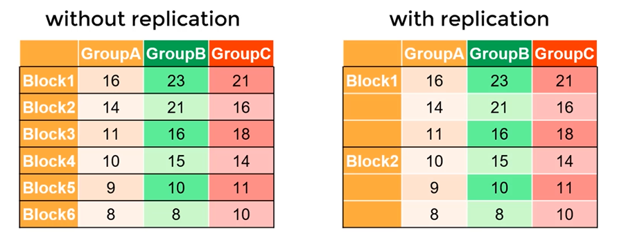
ANOVA (Analysis of Variance)
Regression
- The goal of regression is to develop an equation or formula that best describes the relationship between variables
- Go from data points to a function that approximates as passes (or approximately passes) for those data points
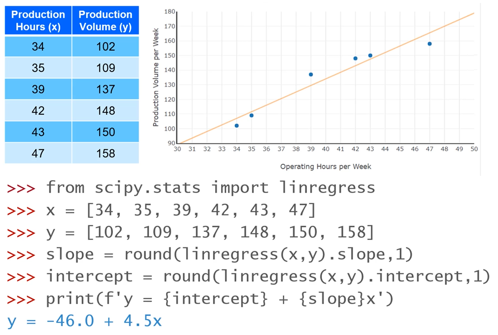
Linear regression
- Linear regression attempts to find the line that best describes our data by minimizing the Squared Error using the means of our data ($\bar x, \bar y$) and each point of our data ($x_i,y_i$)
- Linear regression has limitations since only relies on lineal equation
$$\hat y = b_0 + b_1x$$
$$b_1 = \dfrac{\sum_{i=1}^N (x_i-\bar x)(y_i-\bar y)}{\sum_{i=1}^N (x_i-\bar x)^2}$$
$$b_0 = \bar y-b_1 \bar x)$$
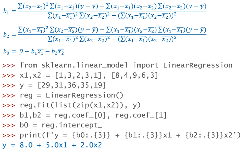
Multiple regression
- Multiple regression lets us compare several independent variables to one dependent variable at the same time
$$\hat y = b_0 + b_1 x_1 + b_1 x_2 + \cdots + b_n x_n$$
Chi-Square Analysis
The goodness of fit: are the observed results straying/deviating too far way from the expected results
Chi-Square test ($\chi^2$) is used to determine the probability of an observed frequency of events given an expected frequency
- low $\chi^2$ means a high correlation of observed and expected values
- higher $\chi^2$ means a observed values are deviating from expected values
- Assumes outcomes are independent of each other so it an outcome is what we expect or not does not affect following outcomes
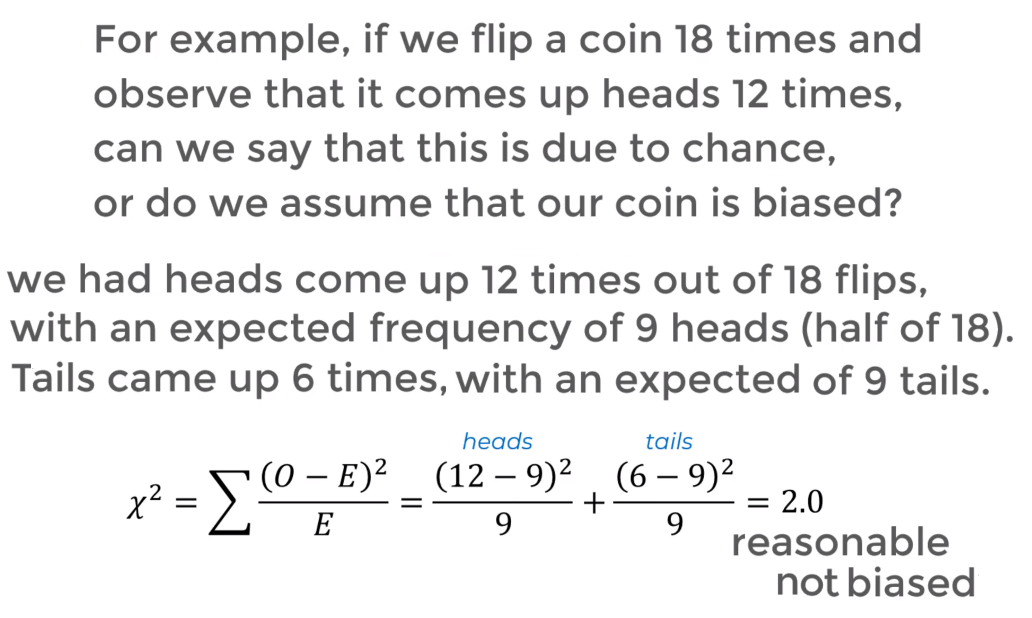
Formula: $\chi^2 = \sum \dfrac{(O-E)^2}{E}$
- $O$: Observed values
- $E$: Expected values
- $df = N_{\text{possible outcomes}} - 1$: Number of different expected values minus 1
References