This will help me create more stuff and fix the existent content...
Python Data & Analysis Tools for Finance
Finance Fundamentals
Portfolio Basics
A Portfolio is a set of allocations in a variety of assets. In order words is a set of weighted assets. E.x. you have 0.1 of your money in BTC, 0.2 in AMZN stocks, 0.3 in AAPL stocks and 0.4 in an ETF
Key statistics in a portfolio
Daily Returns The percent return from 1 day to the next
Normalized return The percent return from the day we started the investment to a certain day. Formula $N_R = \dfrac{\text{Current Stock price}}{\text{Stock price at day of investment}}$
Cumulative Return The amount returned after a certain time period
Avg. Daily Return Mean of the daily returns over a period of time (E.x. 15, 30 days)
STD Daily Return Standard Deviation of daily returns (Volatility of the daily return)
Quantifies the relationships between mean daily return and the std. daily return (volatility)
It is a measure of risk or more formally a measure of the risk-adjusted return
Formula $SR = \dfrac{R_p - R_f}{\sigma_p}$
$R_p$ Expected portfolio return
$R_f$ Risk-free return: return you would receive in a risk-free investment (E.x. bank account with constant return)
$\sigma_p$ Portfolio standard deviation
Annualized Sharpe Ratio (ASR):
Allow an investors to analyze how much greater a return he is obtaining in relation to the level of additional risk taken to generate that return.
ASR values around >=1 are considered good values, around >=2 is very good and >=3 is considered excellent
If you have daily data and want to get annual data you need to perform following conversions
Daily: $ASR = \sqrt{252} \cdot SR$
Weekly: $ASR = \sqrt{52} \cdot SR$
monthly: $ASR = \sqrt{12} \cdot SR$
Optimize holdings
Randomly guessing and checking allocations based on a the values of another statistics in general is known as Monte Carlo Simulation
E.x. We randomly assign weight to each asset in our portfolio, then we calculate daily return mean and STD of daily return and see which combinations gives us better results by evaluating the SR and ASR. We can plot return vs SR or ASR to see which combination gives betters results (there is 1-to-1 map between ASR & SR to a combination of allocations)
Minimization its just finding the value of independent variable ($x$) that gives us the minimum value of the dependent variable ($y$)
E.x. What value of $x$ minimize $y$ in equations 1) $y=x^2$ the answer is $x=0$ which gives a $y=0$ and 2) $y=(2-x)^2$ the answer is $x=20$ which gives a $y=0$
Finding the optimal value for a metric can be done using Optimization algorithm which are based on Minimization
We want to maximize Sharpe Ratio which means we can create an optimizer that attempts to minimize the negative Sharpe Ratio (inverse)
Border/Efficient Frontier indicates the highest return for a certain value of volatility
Liquidity refers to how easy can you get your money in and out of an investment, high liquidity means it is very easy, low liquidity means it is hard or you need to wait for a certain period of time until a contract date is reached for example
An investment mechanism made of a pool of other funds (money) collected from many investors for the purpose of investing in stocks, bonds, other market instruments or any other assets
These are operated by money manager who is responsible of investing the fund's capital and attempting to produce gains for fund's investors
They usually need to disclose they holdings every certain time but this can vary (More less transparent)
Liquidity: medium - Buy/Sell at end of the day through a broker
Aggressive/Risky investment mechanism that uses pooled funds and employ multiple strategies to earn as much returns (alpha=returns) as possible for their investors
Usually only accessible to accredited investor
Don't need to disclose holdings to the public or investors (Not so transparent)
Liquidity: low - Depends on agreement (could be every week month, 6 months year, etc)
Fee: 1% or 2% fund and 10 or20% of profits (2 & 20 rule or 1 & 10 rule)
Some stocks pay Dividends, so for each stock a shareholder has, he receives some payout at certain defined date, this usually cause price to jump before dividend announcement and then drop after dividend pay out
Stock Splits usually occur if the price of an individual stock become really high, so a company creates a ratio split (e.g. 2:1, 3:1, 4:1, 5:1) this is the reason the Adj. Close price exists, which adjusts the historical prices to match up and take into account the stock splits, also takes into account dividends. This is the reason it is important to use adjusted close/open prices for historical analysis
Survivorship Bias: if you are using S&P500 as an indicator the time period you pick can matter since the list of companies has changed trough the years
EMH (Efficient Market Hypothesis) is an investment theory that stats it is impossible to "beat the market" so it is not possible for trades to purchase undervalued stocks or sell stocks for inflated prices
Order & Order Books
When you want to buy or sell and asset what is happening is that you are creating an Order in a broker, then it goes to an exchange (or multiple exchanges), once the exchange receives the order it goes in to an Order Book which is just a list of Buy and sell orders
Order Information:
Buy or sell action type
Symbol: pair to trade
Number of shares or assets
Fulfill type: LIMIT, MARKET, etc.
Price (only needed for LIMIT or other types)
Orders Scenarios:
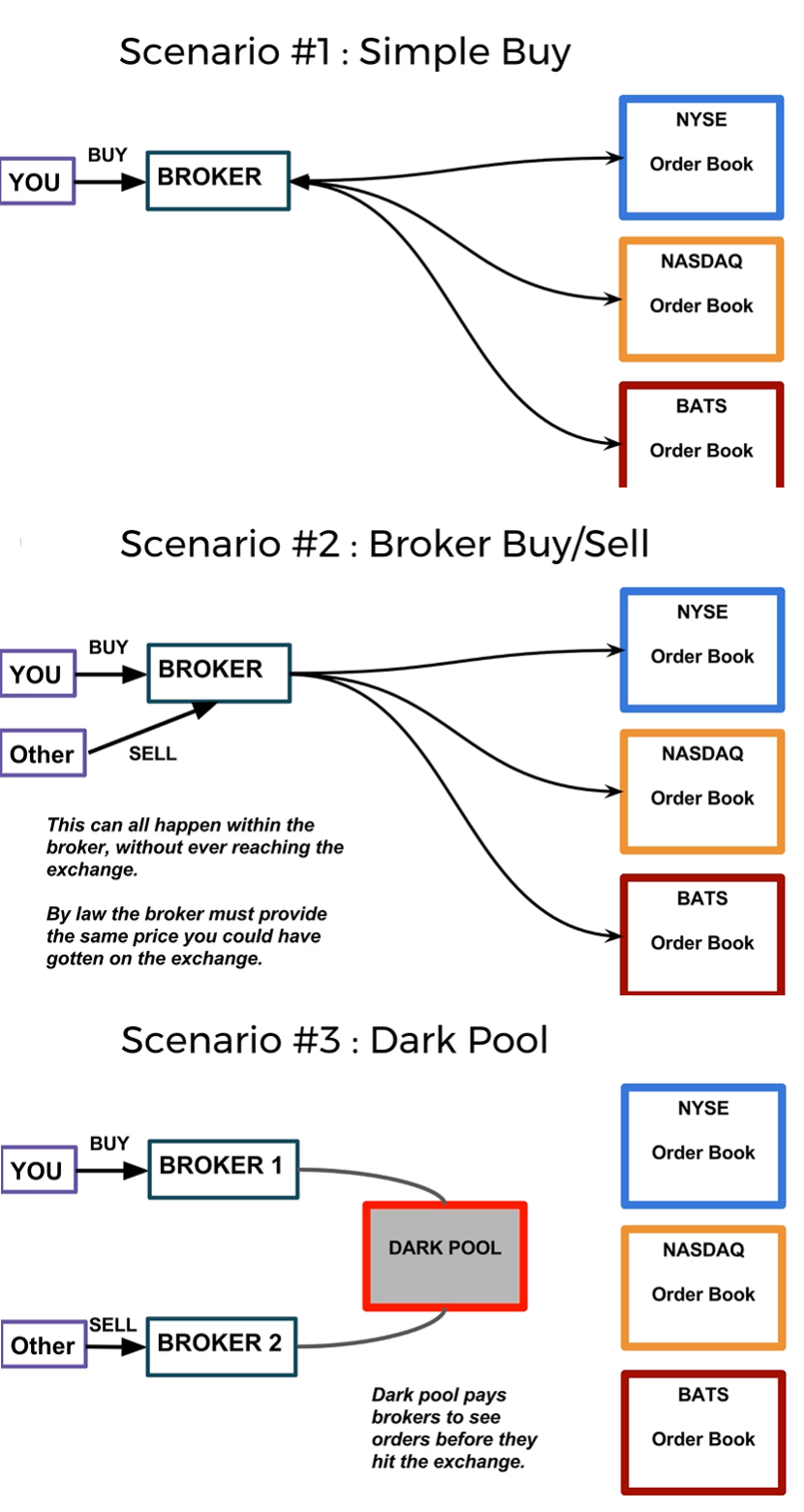
You say you want to buy an asset that goes to the broker, then to the exchanges
You say you want to buy an asset other client of the same broker says he wants to sell that same asset so the transaction can be kept internal by the broker but usually by law broker also has to guarantee you get the same price you could have gotten in exchange
You say you want to buy an asset other client on a different broker says he want to sell that same assets, it can happen that brokers use and intermediary (a dark pool) so the trade never gets to exchanges but it is performed
Dark pool It is a private exchange that pays brokers to see orders before they hit the exchange, although it looks shady it can work as protection if you want to make a massive trade once it hits the exchange it is public so buyers and sellers there can rapidly change to benefit from your trade.E.x. You say you want to sell 1 billion of certain stock since order is so big if it reaches the exchanges while it is being fulfilled sellers of that stock can start increasing their sell price which makes you pay more for what you want to buy
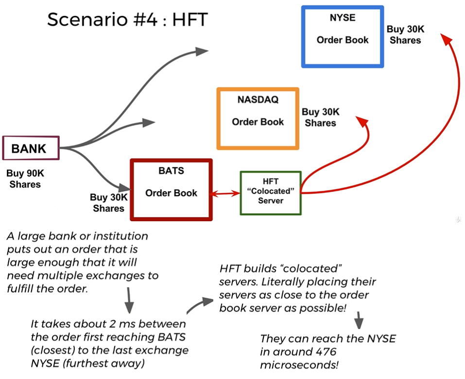
High Frequency Trading (HFT) or Latency Arbitrage
Technique to try to take advantage of latency differences due to geographical distances (Times are in order of microseconds)
Affects or works only large orders that need to be divided between exchanges in order to be fulfilled. In other words it happens when you put a large order that requires multiple exchanges to fulfill the order
General process
You put an order for 90 stocks at certain price 2. Because it is a large order it is divided between 3 exchanges but the whole order information is disclosed. E.x. it says I will buy 30 stocks on first exchange but this is part of larger order of 90 stocks
It reaches first exchange at a certain time (time 0) with all the information but will reach last exchange after 2 ms of that
If there is a HFT server close to first exchange it knows there will be other 2 orders of 30 stocks each in the other exchanges
Since this HFT server now knows it will take you 2ms to reach last exchange and also using technology to reach that exchange faster (wave towers, direct fiber, etc) it buys the stock at market price then puts a sell order specifying a sell price just a little higher to what it just paid
Once you reach the last exchange you end up buying stocks from the server that just bought the shares and right after that placed a sell order
It is a technique that allows you to profit if a stock drops in price
It comes with great risk because there could be no limit to the amount of you can lose
The Short selling transactions happen through a broker that works as intermediary. General process:
A certain stock is currently valued at 500 USD you think it will drop and somebody has 10 shares of this stock
You borrow the 10 stocks from that somebody promise to return the stocks at a future date
You sell the shares and get 5000 USD, then place an order to buy 10 stocks at 100 USD each (invest 1000 USD total)
Scenarios:
4.a) You are correct and your order is fulfilled now you have back the 10 stocks so you return those stocks and also you have 4000 USD that you can keep and everybody is happy
4.b) You are wrong and now each stock costs 1000 USD so your order is not fulfilled and the date when you said you will return the stocks has passed so you need to buy stocks at this higher price (need to take 10000 USD out of your pocket) to return the stocks
CAPM
The Capital Assets Pricing Model (CAPM) is a model that help describe risk and also helps to separate market return vs your portfolio return
We can define the return of a portfolio at some time $t$ as the following formula for $r_p(t)$ where:
$n$: Number of assets, securities or stocks
$w_i$: Weight of a particular asset $i$
$r_i(t)$: Return of a particular asset $i$ at time $t$
$$r_p(t) = \sum_{i=1}^n w_i r_i(t)$$
We can also image the whole market as a portfolio where the weight can be obtained using the market cap (Total number of shares * price of share), de dive by the whole market cap of the market which can be obtained by summing all the market caps
The CAPM equation describes the return of an individual stock $i$, it states the return of a given stock is defined by the entire market multiplied by a particular factor for this stock $\beta_i$ plus an adjustment or residual factor $\alpha_i(t)$ which is random and cannot be predicted but it can be considered zero or close to zero for CAPM (in other words that it can be ignored)
$r_i(t)$ Return of particular asset $i$ at time $t$
$r_m(t)$ Return of entire market at time $t$
$\beta_i$ Market factor. For example if $\beta_i=1$ means asset moves in line with market, if $\beta_i=2$ means it moves up and down twice as much as the market
$\alpha_i(t)$ adjustment factor that is considered zero or very close to zero in CAPM
$$r_i(t) = \beta_i r_m(t) + \alpha_i(t)$$
In general what CAPM model is expressing is that there is some relationship between our portfolio return and the overall market return, this relationship is $\beta_i$ and we can express this as:
$$r_p(t) = \beta_i r_m(t) + \alpha_i(t)$$
import os
import datetime
from scipy import stats
import pandas as pd
import pandas_datareader as web
import matplotlib.pyplot as plt
import numpy as np

base_path = "."
SYM = "AMZN"
stock = pd.read_csv(os.path.join(base_path, "{}.csv".format(SYM)), index_col='Date', parse_dates=True)
spy_etf = df = pd.read_csv(os.path.join(base_path, "SPY.csv"), sep=",", index_col='Date', parse_dates=True)

#stock["close"].plot(label=SYM)
#spy_etf["Close"].plot(label="SPY ETF")

stock["cumulative"] = stock["close"]/stock["close"].iloc[0]
stock["daily return"] = stock["close"].pct_change(1)
spy_etf["Cumulative"] = spy_etf["Close"]/spy_etf["Close"].iloc[0]
spy_etf["Daily Return"] = spy_etf["Close"].pct_change(1)

# Compare cumulative returns
# stock["cumulative"].plot(label=SYM)
# spy_etf["Cumulative"].plot(label="SPY ETF")

# Check correlation, if there is high correlation we expect to see a line
# plt.scatter(stock["daily return"], spy_etf["Daily Return"], alpha=0.25)

# High beta means asset behaves pretty much like the market
beta, alpha, r_value, p_value, std_err = stats.linregress(stock["daily return"].iloc[1:], spy_etf["Daily Return"].iloc[1:])
print("CAPM for {}\nbeta".format(SYM), beta, "\nalpha", alpha, "\nr_value", r_value, "\np_value", p_value, "\nstd_err", std_err)

# Simulate a stock that behaves a lot like the market
noise = np.random.normal(0, 0.001, len(spy_etf["Daily Return"].iloc[1:]))
fake_stock = spy_etf["Daily Return"].iloc[1:] + noise
beta, alpha, r_value, p_value, std_err = stats.linregress(fake_stock, spy_etf["Daily Return"].iloc[1:])
print("CAPM for fake stock\nbeta", beta, "\nalpha", alpha, "\nr_value", r_value, "\np_value", p_value, "\nstd_err", std_err)
# plt.scatter(fake_stock, spy_etf["Daily Return"].iloc[1:], alpha=0.25)

# print(stock.head())
# print(spy_etf.head())

# plt.legend()
# plt.show()
Algorithm Trading on a Trading platform
Blueshift® is a platform that allows coders to write, test and backtest investment algorithms
initialize:
Called once when our algorithm starts
Requires context as input
context is an object which is basically an extender dictionary used to maintain the status of your algorithm during the backtest or live trading
Used instead of global variables
handle_data:
Called once at the end of each minute
Requires context and data as inputs
data object with methods to adjust portfolio and check historical data
from datetime import datetime
AAPL = 0
CSCO = 1
AMZN = 2
IBM = 3

# Zipline
from zipline.api import(    symbol,
                            order_target_percent,
                            schedule_function,
                            date_rules,
                            time_rules,
                            record
                       )

def initialize(context):
    """
        A function to define things to do at the start of the strategy
    """
    context.tech_stocks = [symbol("AAPL") , symbol("CSCO"), symbol("AMZN"), symbol("IBM")]

    ## Uncomment one of the following sets
    # 1 Record
    schedule_function(rebalance, date_rules.every_day(), time_rules.market_open())
    schedule_function(record_vars, date_rules.every_day(), time_rules.market_close())

    # 2 schedule to do something witha certain frequency, like adjust portfolio
    #schedule_function(open_positions, date_rules.week_start(), time_rules.market_open())
    #schedule_function(close_positions, date_rules.week_end(), time_rules.market_close())

def rebalance(context, data):
    order_target_percent(context.tech_stocks[AMZN], 0.5)
    order_target_percent(context.tech_stocks[IBM], -0.5) #Short sell ibm

def record_vars(context, data):
    record(amzn_close=data.current(context.tech_stocks[AMZN], 'close'))
    record(ibm_close=data.current(context.tech_stocks[IBM], 'close'))

def open_positions(context, data):
    order_target_percent(context.tech_stocks[AAPL], 0.1)

def close_positions(context, data):
    order_target_percent(context.tech_stocks[AAPL], 0)

def handle_data(context, data):
    print(datetime.now().strftime("%d/%m/%Y %H:%M:%S"))
    print(data.is_stale(symbol("AAPL")), data.can_trade(symbol("AAPL")))
    price_history = data.history(context.tech_stocks, fields="price", bar_count=5, frequency='1d')
    print(price_history)
    tech_close = data.current(context.tech_stocks, 'close')
    print(type(tech_close))
    print(tech_close)
    print("-"*15 + "\n")
Pairs Trading is a strategy that takes two or more securities we believe are paired or related to each other in some way (e.g. Pepsi and coca-cola, two airlines, two retail companies, etc.) and creates an algorithm based on that relationship
A general way to know if they is a relation ship is to plot them ads see if the graphs look similar or get their correlation matrix np.corrcoef(series1, series2) and see if their correlation coefficient is close to 1
price trading makes the assumption that changes in spread are trading opportunity
Trading platforms pipelines are sued for algorithms that follow a structure (set of steps you need to perform in a certain order). Pipelines provide an API to implement the general structure of the algorithms which is:
Compute scalar values for all assets (for example 20 MAVG)
Select a smaller set of assets based on the values computed in previous step
Set/adjust desired portfolio weights on the selected assets
Place orders on assets to reflect selection and desired weights
Classifier is a function that transforms the input of an asset and a timestamp to a categorical output. e.x. taking AAPL and 2017 as inputs and returns it belongs to tech sector
A Factor is a function that takes in an asset and a timestamp and returns a numerical value such as the 20 day Moving Average
Filters take in an asset and timestamp and return a Boolean while Screens allows you to actually select rows where that filter is true and Masking allows you to ignore assets, the main differences with screens is that masks take place at the beginning and screens & filters take place at the end
Leverage is the ability to borrow money for use in investing, in trading it can be seen as reinvesting bet to gain a greater return on our investment
Leverage is usually provided by the broker (Terms and conditions depend on the broker)
Measured in terms of ratio (the sum of your bet and capital divided by your capital base) \text{Leverage Ratio} = (\text{Debt} + \text{Base Capital})/\text{Base Capital}
Sentiment Analysis uses NLP (Natural Language Processing) to attempt to detect sentiment in some text
Examples of Sentiment Analysis:
"This is bad! It is going to fail" -> Negative sentiment
"Awesome! Good job you will win" -> Positive sentiment
Impact is a measure of how likely a stock price will change as a result of the sentiment, usually goes from 0 to 100 while Sentiment goes from -1 (negative) to 1 (positive)
Forward Contracts are an agreement between two parties to pay a delivery price $K$ for some asset at some future time while the actual market price at time of that asset is $S_T$
The person selling is in the short position while the person buying it in the future time is in the long position
Pay off for long position is $S_T-K$
Pay off for short position is $K-S_T$
These contract actually reduces risk on both sides because parties know how much price will be in the future but depending on how the contract is defined parties need to wait until contract matures to execute transactions (lack of liquidity)
Example: Bill (long position, he thinks price will go up) agrees to pay Sandy (short position, she thinks price will go down) 100 USD in one year from now for a barrel of gasoline, the one who wins depends on the price of gasoline. One year passes scenarios:
Price of barrel of gasoline is 150USD so Sandy lost potential profit and Bill save up 50USD
Price of barrel of gasoline is 50USD so Sandy gets more profit and Bill ends up paying an extra 50USD
derivatives are contracts between two or more entities, the value of the contract is based on an agreed-upon underlying financial asset (like a stock, market index, currency, etc)
Futures
They re an example of a simple derivative
They are forward contracts that have standardized for trade on an exchange, this means the exchange is a third entity that handles the transaction and manages the contract
The only difference between a futures contract and a forward contracts is the exchange that acts as a middle man
They are defined daily based on the price of the underlying asset which increases or decreases the amount of money in a margin account