Python Data & Analysis Tools

numpy

numpy arrays

• numpy Numerical Python is a library that allows us to generate and handle data

• Numpy uses an object/structure referred to as numpy array (numpy.ndarray) that can store data efficiently and execute functions on that data (better than built-in python list)

• install

  • pip: pythom -m pip install numpy

• numpy arrays can be vectors (one-dimensional arrays) or matrices (two-dimensional arrays)

• In numpy a number followed by a dot . indicates it is a floating point number. e.x. [0., 0., 1.]

• arange generates an array from start to end but not including and lispace generates an array with exactly the number of elements specified and evenly spaced

• Numpy has a great variety of functions and distributions to generate random numbers

import numpy

# Create Numpy Array from python list
print("numpy array")
np_array = numpy.array([1, 2, 3])
print(type(np_array), np_array)

# Create Numpy matrix from python list of lists
print("numpy matrix")
np_matrix = numpy.array([[1, 1, 1], [2, 2, 2], [3, 3, 3]])
print(type(np_matrix))
print(np_matrix)

# numpy arange to generate arrays
print("numpy arange")
np_ar1 = numpy.arange(0, 5, 1)
np_ar2 = numpy.arange(0, 5, 0.5)
print(np_ar1, np_ar2)

# Create array or matrix of zeros
print("numpy zeros")
zeros = numpy.zeros(4)
print(zeros)

# Create array or matrix of ones
print("numpy ones")
ones = numpy.ones((2, 3))
print(ones)

# numpy linspace to generate evenly spaced numbers
# over specified interval
print("numpy linspace")
np_lin1 = numpy.linspace(0, 4, 5)
np_lin2 = numpy.linspace(0, 4.5, 6)
print(np_lin1, np_lin2)

# Create identity matrix
print("identity matrix")
eye = numpy.eye(3)
print(eye)

# Creates array with random samples
# of uniform distribution [0, 1)
# every number has the same probability of being picked
print("uniform distribution")
uni_rand1 = numpy.random.rand(1)
print(uni_rand1)
uni_rand2 = numpy.random.rand(4)
print(uni_rand2)
uni_rand3 = numpy.random.rand(3, 3)
print(uni_rand3)

# Creates array with samples from a
# standard normal distribution [0, 1)
# the closer you are to the zero the higher probability of the number being picked
print("standard normal distribution")
snor_rand1 = numpy.random.randn(1)
print(snor_rand1)
snor_rand2 = numpy.random.randn(4)
print(snor_rand2)
snor_rand3 = numpy.random.randn(3, 3)
print(snor_rand3)

# Random integer up to but not including high
print("random integers")
int_rand = numpy.random.randint(low=1, high=10+1)
print(int_rand)
int_rand_array = numpy.random.randint(low=1, high=10+1, size=5)
print(int_rand_array)

# generate always same random data with seed
numpy.random.seed(101)
print(numpy.random.rand(1))
print(numpy.random.rand(1))

# reshape array to a VALID dimension
print("reshape arrays")
orig_array = numpy.arange(0, 6)
print(orig_array, "shape", orig_array.shape, "storing", orig_array.dtype,
      "max", orig_array.max(), "at index", orig_array.argmax())
print(orig_array.reshape(2, 3))  # numbers here must multiply to size of original array
print(orig_array.reshape(1, 6))
print("shape", orig_array.reshape(6, 1).shape)
print(orig_array.reshape(6, 1))

• Python indexing and slicing apply to numpy arrays but numpy also allows to do broadcast which means reassignment of values to the array or certain range of the array (arr[0:5] = 100)

  • assignment of certain range will only give a reference to those values in the array so changes affect original array, you can user copy() method to explicitly copy

• numpy supports [r][c] or [r,c] indexing for matrixes

• Conditional selection used to grab elements from an array based on some operator by creating an numpy array of booleans arr[arr > 4]

import numpy as np

# Array slicing
arr = np.arange(0, 11)
print("arr", arr)
arr[1:5] = 100
print("reassign", arr)

arr = np.arange(0, 11)
slice_of_arr = arr[1:6]
print("slice_of_arr", slice_of_arr)
slice_of_arr[:] = 99
print("slice_of_arr reassign", slice_of_arr)
print("reassign", arr)

# Matrix slicing and indexing
mat = np.arange(9).reshape(3, 3)
print("mat")
print(mat)
print("mat[1][2]", mat[1][2])
print("mat[1,2]", mat[1, 2])
print("row 1 = mat[1]", mat[1])
print("mat[:2,1:]") ; print(mat[:2, 1:])
print("mat[1:,:2]") ; print(mat[1:, :2])
print("mat.sum") ; print(mat.sum(axis=0))  # axis: 0=rows/vertical, 1=cols/horizontal

# Conditional selection
arr = np.arange(1, 11)
bool_array = arr > 4
print("arr > 4", bool_array)
print("arr[bool_array]", arr[bool_array])
print("arr[arr>=9]", arr[arr <= 9])
print("arr[arr<=0]", arr[arr <= 0])

numpy operations

• Usually behave element by element operations
• numpy usually returns a warning and nan on indeterminations like 0/0 and inf for a number divided by zero or -inf for other indeterminations but it does perform the operations

import numpy as np

arr = np.arange(0, 10)

print("sum", arr+arr)
print("mul", arr*arr)
print("div", arr/arr)
print("inv", 1/arr)
print("pow", arr ** 2)
print("sum scalar", arr+100)
print("sqrt", np.sqrt(arr))
print("exp", np.exp(arr)) # e to the power of each element of the array
print("sin", np.sin(arr))
print("log", np.log(arr))

Pandas

• Pandas (PANel-DAta) is a data analysis library built off of numpy created to help with datasets specially finance data

• Pandas features:

  • Provides a fast and efficient DataFrame Object used for data manipulation, this object also has integrated indexing
  • Provides Tools for reading and writing data between in memory data structures and different formats like CSV files, text, files, Excel Files, SQL databases, HDF5 format, etc
  • It is great interaction with visualization Python libraries
  • Pandas is highly optimized for performance, critical code paths are written un Cython or C
  • It can transform or aggregate data

• Pandas Series are arrays (or numpy arrays) than can be indexed by a named index, datetime index or any object index instead of just numerical index. They are one-dimensional numpy.ndarray with axis labels

import numpy as np
import pandas as pd

labels = ['a', 'b', 'c']
my_list = [0, 10, 20]
arr = np.arange(0, 30, 10)

print("Series from list use default index")
my_series = pd.Series(data=my_list)
print(type(my_series))
print(my_series)

print("Series from list with labels")
my_series = pd.Series(data=my_list, index=labels)
print(my_series)

print("Series from numpy ndarray with labels")
my_series = pd.Series(data=arr, index=labels)
print(my_series)

print("Series from any iterable list of objects")
my_series = pd.Series(data=[sum, max, len, all])
print(my_series)

print("Series from strings")
my_series = pd.Series(data=labels)
print(my_series)

print("Series from dict")
ser1 = pd.Series(data={'apple': 7, 'orange': 4, 'banana': 5})
ser2 = pd.Series(data={'apple': 3, 'watermelon': 1})
print("Series index as dict", ser1["apple"])
print("Adding series by default sums ONLY where there is a match")
print(ser1+ser2)

DataFrames

• DataFrames are built on top of Pandas Series objects (pandas.core.series.Series), they are a collection of series, a DataFrame has rows and columns where each column is a series and each row is also a series

• DataFrame are just fancier numpy matrixes where axis=0 refers to the rows and axis=1 refers to columns

import numpy as np
import pandas as pd
from numpy.random import randn
np.random.seed(101)

data = randn(5, 4) # 5 rows 4 columns
rows =  ['A', 'B', 'C', 'D', 'E'] # 5 rows
columns =  ['W', 'X', 'Y', 'Z']   # 5 columns

# each column is a series
df = pd.DataFrame(data=data, index=rows, columns=columns)
print("DataFrame")
print(type(df))
print(df)

print("Get a column = Get a series")
print(type(df['W']))
print(df['W']) # pass column name as index
# print(df.W) # also possible but no recommended to avoid accesing series methods

print("Get multiple columns = Get multiple series = Get a subset DataFrame of original DataFrame")
print(df[['W', 'Z']])
print("Get just certain rows of all columns in a DataFrame")
print(df.iloc[0:3])

print("Add/Append a columns to DataFrame")
df['V'] = df['W'] + df['Y']
df['T'] = pd.Series(data={'A': 1, 'B': 2, 'C': 3, 'D': 4, 'E': 5})
print(df)

print("Remove columns from DataFrame")
df.drop('V', axis=1) # by default just return resulting dataframe but doesn't affect original
df.drop('T', axis=1, inplace=True) # set inplace to affect original dataframe
print(df)

print("Remove rows from DataFrame")
print(df.drop('E', axis=0))

print("Get a row = Get a series")
print(type(df.loc['A']))
print(df.loc['A']) # row name
print(df.iloc[0]) # row index

print("Get element from DataFrame")
print(type(df.loc['B', 'Y']))
print(df.loc['B', 'Y'])

print("Get subset of DataFrame")
print(type(df.loc[['A', 'B'], ['W', 'Y']]))
print(df.loc[['A', 'B'], ['W', 'Y']])

• DataFrames allow conditional selection for multiple conditions we need ot use & and | instead of and and or due to overloading of operators

• If you pass a series of Boolean values (for example a column with comparison operators df["W"]>0) you will get rows where the series happened to be true

import numpy as np
import pandas as pd
from numpy.random import randn
np.random.seed(101)

data = randn(5, 4) # 5 rows 4 columns
rows =  ['A', 'B', 'C', 'D', 'E'] # 5 rows
columns =  ['W', 'X', 'Y', 'Z']   # 5 columns

# each column is a series
df = pd.DataFrame(data=data, index=rows, columns=columns)
print("DataFrame conditional selection")
print(df[df > 0])

print("DataFrame conditional columns selection")
print(df[df["W"] > 0])
print("DataFrame conditional selection chained to access")
print(df[df["W"] > 0]["X"])
print("DataFrame multi conditional selection")
print(df[(df["W"] > 0) & (df["Y"]>1)])
# print(df[(df["W"] > 0) | (df["Y"]>1)])

print("DataFrame reset index to integers")
print(df.reset_index()) # needs inplace to affect original

print("DataFrame set new index")
new_rows = ["F", "G", "H", "I", "J"]
df["new"] = new_rows
print(df.set_index(keys="new")) # needs inplace to affect original
print(df)

• We can create dataframes with an index hierarchy which means an index with multiple levels (multi-level index)

import numpy as np
import pandas as pd
from numpy.random import randn
np.random.seed(101)

outside =  ['G1', 'G1', 'G1', 'G2', 'G2', 'G2']
inside =  [1, 2, 3, 1, 2, 3]

print("Create MultiIndex object from list of tuples")
hier_index = list(zip(outside, inside))
print(type(hier_index), hier_index)
hier_index = pd.MultiIndex.from_tuples(hier_index)
print(hier_index)

print("Create multi-level dataframe")
df = pd.DataFrame(data=randn(6, 2), index=hier_index, columns = ['A', 'B'])
print(df)

print("Get subset dataframe with an index level")
print(df.loc["G1"])
print("Get subset dataframe with chained index level")
print(df.loc["G1"].loc[2])

print("Set names for indexes")
df.index.names = ['Groups', 'Numbers']
print(df)

print("Get element on multi level index dataframe")
print(df.loc["G2"].loc[2]["B"],"=",df.loc["G2"].loc[2].loc["B"])

print("Get cross section of rows or columns")
print(df.xs(key="G1"))
print(df.xs(key=1, level="Numbers"))

• We can create Dataframes from dictionaries where keys will be the columns and each key must have a list (of equal size) that represent the data values, you can pass a list of index equal to the size of these lists to set specific index

• DataFrames access are always from top to bottom, from outer to inner indexes,from outer columns to last inner column, then from outer rows (indexes) to inner indexes

import numpy as np
import pandas as pd

d = {"A": [1,2, np.nan], "B": [7,np.nan,np.nan], "C": [4,5,6]}

df = pd.DataFrame(data=d)
#df = pd.DataFrame(data=d, index=["a", "b", "c"])
print(df)

print("Drop any row with missing values")
print(df.dropna(axis=0))

print("Drop any columns with missing values")
print(df.dropna(axis=1))

print("Drop based on threshold (number of NaN values) / keep rows with 2 or more valid values")
print(df.dropna(axis=0, thresh=2))

print("Fill missing values")
print(df.fillna(value=df['A'].mean()))

• Pandas GroupBy can be seen as the Filter By column in Excel

• Pandas GroupBy functionality allows you to group multiple rows by the values in a certain column and then perform an operation to combine those values

• groupby returns a pandas.core.groupby.generic.DataFrameGroupBy object, methods of this object by default ignore non numeric columns and return DataFrame objects where the indexes are the values from the column yo passed to groupby

• GroupBy lets you choose a column to group by values, gathers all those rows based off the same or other column and then performs an aggregate function on those values

  • aggregate function is just any function that operate on a collection of values and returns a single value for example a sum of the values, average of the values, standard deviation of the values, etc

import numpy as np
import pandas as pd

d = {
     "Company": ['GOOG','GOOG','MSFT','MSFT','FB','FB'],
     "Person": ['Sam', 'Charlie', 'Amy', 'Vanessa', 'Carl', 'Sarah'],
     "Sales": [200,120,340,124,243,350]
}

df=pd.DataFrame(data=d)
print(df)

byCompany = df.groupby("Company")
print(type(byCompany))

print("Get mean sales by company")
print(byCompany.mean())

print("Get std sales by company")
print(byCompany.std())

print("Get sum sales by company")
print(byCompany.sum())

print("Get sum sales of a certain company")
print(df.groupby("Company").sum().loc['GOOG'])

print("Count number of instances")
print(byCompany.count())

print("Get Max/Mins")
print(byCompany.max())
#print(byCompany.min())

print("Get Describe")
descdf = byCompany.describe()
print(descdf)
print("Specific mean value", descdf["Sales"]["mean"]["FB"])

print("Get Describe transposed")
tdf = byCompany.describe().transpose()
print(tdf)
print("Specific mean value", tdf["FB"]["Sales"]["mean"])

• Pandas provides 3 main ways of combining DataFrames
  • Concatenating (pd.concat([df1, df2])): Combine DataFrames, dimension should match along the axis to concatenate (axis=0 -> add rows so we must have same number of columns)
  • Merging (pd.merge(left, right, how='inner', on='key')): Merges data frames like merging DB SQL tables which means concatenate based on a key column they share
  • Joining : used to combine columns of two dataframes can have different indexes, it is same as merge except keys are on the index instead of in a column

Concatenate can add rows or columns, join and merge usually adds columns but in general it can add both at the same time

import numpy as np
import pandas as pd

df1=pd.DataFrame(data={
     "A": ['A0','A1','A2','A3'],
     "B": ['B0','B1','B2','B3'],
     "C": ['C0','C1','C2','C3'],
     "D": ['D0','D1','D2','D3']
}, index=[0, 1, 2, 3])

df2=pd.DataFrame(data={
     "A": ['A4','A5','A6','A7'],
     "B": ['B4','B5','B6','B7'],
     "C": ['C4','C5','C6','C7'],
     "D": ['D4','D5','D6','D7']
}, index=[4, 5, 6, 7])

df3=pd.DataFrame(data={
     "A": ['A8','A9','A10','A11'],
     "B": ['B8','B9','B10','B11'],
     "C": ['C8','C9','C10','C11'],
     "D": ['D8','D9','D10','D11']
}, index=[8, 9, 10, 11])

#print(df1) ; print(df2) ; print(df3)

print("Concatenate along axis=0 (add rows)")
print(pd.concat([df1, df2, df3], axis=0))

print("Concatenate along axis=1 (add columns)")
print(pd.concat([df1, df2, df3], axis=1))

left=pd.DataFrame(data={
     "A": ['A0','A1','A2','A3'],
     "B": ['B0','B1','B2','B3'],
     "key": ['K0','K1','K2','k3']
})

right=pd.DataFrame(data={
     "C": ['C0','C1','C2','C3'],
     "D": ['D0','D1','D2','D3'],
     "key": ['K0','K1','K2','k3']
})
#print(left) ; print(right)
print("Merge on key")
print(pd.merge(left, right, how='inner', on='key'))

left=pd.DataFrame(data={
     "A": ['A0','A1','A2'],
     "B": ['B0','B1','B2'],
},  index=['K0','K1','K2'])

right=pd.DataFrame(data={
     "C": ['C0','C1','C2'],
     "D": ['D0','D1','D2'],
},  index=['K0','K2','K3'])
#print(left) ; print(right)

print("Join on index")
print(left.join(right))

• Dataframes support multiple useful operations, like creation of pivot tables which are just multi-index out of DataFrame

import pandas as pd

df = pd.DataFrame(data={
    "col1": [1, 2, 3, 4],
    "col2": [444, 555, 666, 444],
    "col3": ['abc', 'def', 'ghi', 'xyz']
})
print(df)

print("Find Unique values in certain column")
print(df['col2'].nunique(), type(df['col2'].unique()), df['col2'].unique())

print("Count values in certain column")
print(type(df['col2'].value_counts()))
print(df['col2'].value_counts())

print("Applies function to column")
print(df['col1'].apply(func=lambda x: x*2))
print(df['col3'].apply(len))

print("Get column and index names")
print(type(df.columns), df.columns)
print(type(df.index), df.index)

print("Sort by column")
print(df.sort_values(by='col2'))

print("Find null values")
print(df.isnull())

df = pd.DataFrame(data={
    "A": ['foo', 'foo', 'foo', 'bar', 'bar', 'bar'],
    "B": ['one', 'one', 'two', 'two', 'one', 'one'],
    "C": ['x', 'y', 'x', 'y', 'x', 'y'],
    "D": [1, 3, 2, 5, 4, 1]
})
print(df)

print("Create Pivot table")
print(df.pivot_table(values='D', index=['A', 'B'], columns=['C']))

• Pandas allows you to do read and write from multiple sources the most common and stable is to use .csv files
  • example .csv file

  a,b,c,d
  0,1,2,3
  4,5,6,7
  8,9,10,11
  12,13,14,15
  

import pandas as pd

in_file = r'.\example.csv'
out_file = r'.\example_out.csv'

print("Read from file to create dataframe")
df = pd.read_csv(filepath_or_buffer=in_file)
print(df)

print("Write dataframe to file ignore index")
df.to_csv(path_or_buf=out_file, index=False)

print("Read from file html")
html_data = pd.read_html('https://www.fdic.gov/resources/resolutions/bank-failures/failed-bank-list/')
print(html_data[0])

print("Read sql, need sql engine installed")
from sqlalchemy import create_engine
engine = create_engine("sqlite:///:memory:")
df.to_sql("my_table", engine)

sqldf = pd.read_sql("my_table", con=engine)

Visualization

• Pandas visualizations components are built on top of Matplotlib

Matplotlib

• It is a Python 2-Dimensional plotting library based of Matlab plotting capabilities, allows to generate plots, histograms, power spectra, bar charts, error charts, scatter plots

• Matplotlib has two API structures you can use

  1. Matplotlib Object Oriented API structure: instantiate figure objects then call methods and attributes from those objects
  2. Matplotlib Functional API structure: just make calls to functions

• A figure in Matplotlib is just like an empty canvas, then add axes setting left bottom and width height percentages in relation to the empty canvas

• Matplotlib allows you to control figure size, aspect ratio and DPI (Dots Per Inch/ Pixels Per Inc)

Simple Functional plot

import matplotlib.pyplot as plt
import numpy as np

x = np.linspace(0, 5, 11)
y = x ** 2

# Functional method to plot
## Simple plot
plt.plot(x, y)
plt.xlabel("x")
plt.ylabel("y")
plt.title("y=x^2")
plt.show()

Simple Functional Subplot

import matplotlib.pyplot as plt
import numpy as np

x = np.linspace(0, 5, 11)
y = x ** 2

# Functional method to plot
## Subplot
plt.subplot(1, 2, 1)
plt.plot(x, y, 'r')

plt.subplot(1, 2, 2)
plt.plot(y, x, 'b')

plt.show()

Object Oriented Simple and Inner plot

import matplotlib.pyplot as plt
import numpy as np

x = np.linspace(0, 5, 11)
y = x ** 2

# Object Oriented method to plot
fig = plt.figure()
# set axis limits left, bottom, width, height
axes = fig.add_axes([0.1, 0.1, 0.8, 0.8])
axes.set_xlabel('x')
axes.set_ylabel('y')
axes.set_title('y = f(x)')
axes.plot(x, y)

fig = plt.figure()

axes1 = fig.add_axes([0.1, 0.1, 0.8, 0.8])
axes1.set_xlabel('x')
axes1.set_ylabel('y')
axes1.set_title('y = x')
axes1.plot(x, y)

axes2 = fig.add_axes([0.2, 0.5, 0.4, 0.3])
axes2.set_xlabel('y')
axes2.set_ylabel('x')
axes2.set_title('x = y')
axes2.plot(y, x)

plt.show()

Object Oriented Subplot

import matplotlib.pyplot as plt
import numpy as np

x = np.linspace(0, 5, 11)
y = x ** 2

# Object Oriented method to subplot
fig, axes = plt.subplots(nrows=1, ncols=2)

# axes is a list we can iterate
for current_axis in axes:
    current_axis.plot(x, y)

# axes is a list we can index
fig, axes = plt.subplots(nrows=1, ncols=2)

axes[0].plot(x, y, 'r')
axes[0].set_xlabel('x')
axes[0].set_ylabel('y')
axes[0].set_title('y = x')

axes[1].plot(x, y, 'b')
axes[1].set_xlabel('x')
axes[1].set_ylabel('y')
axes[1].set_title('y = f(x)')

plt.tight_layout()
plt.show()

Matplotlib plot arguments and attributes

• Matplotlib plot allow you to set
  • Figure Size
  • DPI
  • Color
  • Line Width ('lw')
  • Line Style ('ls')
  • Draw Style ('ds')
  • Markers
  • Axis limits and plot range
  • Labels
  • Location to save a file of figure

import matplotlib.pyplot as plt
import numpy as np

x = np.linspace(0, 5, 11)

# Set figure size, DPI, legends and save figure
width, height = 10, 5
dpi = 100
fig = plt.figure(figsize=(width, height), dpi=dpi)

ax = fig.add_axes([0.1, 0.1, 0.8, 0.8])
ax.plot(x, x ** 3, label='x^3 steps', color='black', ds='steps')
ax.plot(x, x ** 3, label='x^3', color='blue', lw=1, ls='dashed')
ax.plot(x, x ** 2, label='x^2', color='green', lw=2, ls='dashdot')
ax.plot(x, 10*x , label='10x', color='red', ls='solid', marker='o', markersize=5)
ax.plot(x, x, label='x', color='#FF8C00', lw=3, alpha=0.5, ls='dotted')  # RGB Hex Code
ax.set_xlabel('x')
ax.set_ylabel('f(x)')
ax.set_title('f(x) Plot(s)')
ax.legend(loc=(0.05, 0.2))

fig.savefig('my_fig.png', dpi=dpi)
plt.show()

Matplotlib plotting a sine wave

import numpy
import math
import matplotlib.pyplot as plt

def f(x):
    return math.sin(x)

start, stop, step = -2.0*math.pi, 2.0*math.pi, 0.1

x = [i for i in numpy.arange(start, stop, step)]
f_x = list(map(f, x))

plt.plot(x, f_x)
plt.ylabel('f(x)')
plt.xlabel('x')
plt.grid()
plt.xticks([i for i in numpy.arange(round(start), round(stop), 1)])

plt.show()

Matplotlib plotting with no GUI

import numpy as np
import matplotlib
matplotlib.use('agg')
import matplotlib.pyplot as plt

x = np.linspace(0, 5, 11)
fig = plt.figure(figsize=(16, 4))

ax = fig.add_axes([0.1, 0.1, 0.8, 0.8])
ax.plot(x, x ** 3)

fig.savefig('my_fig.png')

Pandas Visualization

• Usually we use the plot method from either a Pandas DataFrame or a Pandas Series object (Columns in a DataFrame are Series, so we can call this directly from a column of the dataFrame)

• install seaborn optionally to format plots automatically. pythom -m pip install seaborn

Pandas plotting with no GUI

import numpy as np
import pandas as pd
import matplotlib
matplotlib.use('agg')
import matplotlib.pyplot as plt

d = {
    "A": [0.039761986133905136, 0.9372879037285884,  0.7805044779316328,  0.6727174963492204,  0.05382860859967886, 0.2860433671280178,  0.4304355863327313,  0.3122955538295512,  0.1877648514121828,  0.9081621790575398],
    "B": [0.2185172274750622,  0.04156728027953449, 0.008947537857148302,0.24786984946279625, 0.5201244020579979,  0.5934650440000543,  0.16623013749421356, 0.5028232900921878,  0.9970746427719338,  0.23272641071536715],
    "C": [0.10342298051665423,0.8991254222382951, 0.5578084027546968, 0.2640713103088026, 0.5522642392797277, 0.9073072637456548, 0.4693825447762464, 0.8066087010958843, 0.8959552961495315, 0.4141382611943452],
    "D": [0.9579042338107532, 0.9776795571253272, 0.7975104497549266, 0.44435791644122935, 0.19000759632053632, 0.6378977150631427, 0.4977008828313123, 0.8505190941429479, 0.530390137569463, 0.4320069001558664]
}
df = pd.DataFrame(data=d)

fig = df[["A", "B"]].plot(figsize=(16,6)).get_figure()
fig.savefig('my_fig.png')

Different types of plots with Pandas

import matplotlib.pyplot as plt
import numpy as np
import seaborn as sns
import pandas as pd
sns.set_theme()

d = {
    "A": [0.039761986133905136, 0.9372879037285884,  0.7805044779316328,  0.6727174963492204,  0.05382860859967886, 0.2860433671280178,  0.4304355863327313,  0.3122955538295512,  0.1877648514121828,  0.9081621790575398],
    "B": [0.2185172274750622,  0.04156728027953449, 0.008947537857148302,0.24786984946279625, 0.5201244020579979,  0.5934650440000543,  0.16623013749421356, 0.5028232900921878,  0.9970746427719338,  0.23272641071536715],
    "C": [0.10342298051665423,0.8991254222382951, 0.5578084027546968, 0.2640713103088026, 0.5522642392797277, 0.9073072637456548, 0.4693825447762464, 0.8066087010958843, 0.8959552961495315, 0.4141382611943452],
    "D": [0.9579042338107532, 0.9776795571253272, 0.7975104497549266, 0.44435791644122935, 0.19000759632053632, 0.6378977150631427, 0.4977008828313123, 0.8505190941429479, 0.530390137569463, 0.4320069001558664]
}
df1 = pd.DataFrame(data=d)

# Plot a histogram from a column (Equivalents, just uncomment one)
df1['A'].hist(bins=5)
#df1['A'].plot.hist(bins=5)
#df1['A'].plot(kind='hist', bins=5)

# Plot an area from a dataframe
df1.plot.area(alpha=0.5)

# Plot an bar plot from a dataframe (Takes index as category)
#df1.plot.bar()
df1.plot.bar(stacked=True)

# Plot line, index will be used for x
# you can add matplotlib arguments like ds, lw, ls, etc
df1.plot.line(y='B', lw=2)

# Plot scatter, using two columns one for 'x' one for 'y'
df1.plot.scatter(x='A', y='B', color="blue")

# Plot scatter, 3 variables one column as color value
df1.plot.scatter(x='A', y='B', c='C', cmap='coolwarm')

# Plot scatter, 3 variables one column as s=size
df1.plot.scatter(x='A', y='B', s=df1['C']*500, color='blue')

# Plot box plot of dataframe
df1.plot.box()

# hexagonal plot (hex get darker as there are more points in them)
df = df1[['A', 'B']]
print(df)
df1.plot.hexbin(x='A', y='B', gridsize=15)

# Kernel density estimation (Equivalents, just uncomment one)
# Kernel density estimation (Equivalents, just uncomment one)
df1["A"].plot.density()
#df1["A"].plot.kde()
#df1.plot.density() # Density estimation fo whole dataframe

plt.show()

Pandas time series visualization

Basic Time series plot with Pandas

import matplotlib.dates as dates
import matplotlib.pyplot as plt
import seaborn as sns
import pandas as pd
sns.set_theme()

from io import StringIO
mc_str = StringIO("""Date,Adj. Close,Adj. Volume\n2007-01-03,31.662754347257,7579100.0\n2007-01-04,31.424579992695,9776100.0\n2007-01-05,31.424579992695,5701000.0\n2007-01-08,31.547275872318,4538500.0\n2007-01-09,31.605015109787,6832800.0\n2007-01-10,31.94423312992,6374800.0\n2007-01-11,32.124668247011,5626900.0\n2007-01-12,31.915363511185,7103000.0\n2007-01-16,32.167972675113,5377700.0\n2007-01-17,32.37727741094,9439700.0\n2007-01-18,32.182407484481,4690400.0\n2007-01-19,32.341190387521,5116900.0\n2007-01-22,32.009189772073,4918000.0\n2007-01-23,32.370060006256,6140200.0\n2007-01-24,31.872059083083,11019000.0\n2007-01-25,31.034840139777,10630200.0\n2007-01-26,30.984318306992,8542300.0\n2007-01-29,31.200840447502,8262100.0\n2007-01-30,31.59058030042,5818200.0\n2007-01-31,32.009189772073,7350900.0\n2007-02-01,32.10301603296,6086700.0\n2007-02-02,32.146320461062,4724100.0\n2007-02-05,32.139103056379,3520900.0\n2007-02-06,32.312320768787,4016600.0\n2007-02-07,32.276233745368,3362000.0\n2007-02-08,32.009189772073,6018400.0\n2007-02-09,32.16075527043,4946700.0\n2007-02-12,32.283451150052,5649800.0\n2007-02-13,32.406147029674,5110800.0\n2007-02-14,32.492755885879,5361000.0\n2007-02-15,32.463886267144,4127300.0\n2007-02-16,32.709278026389,6806600.0\n2007-02-20,33.055713451205,7022100.0\n2007-02-21,33.178409330827,5621200.0\n2007-02-22,33.236148568296,4804000.0\n2007-02-23,33.207278949562,3857700.0\n2007-02-26,33.055713451205,5905200.0\n2007-02-27,32.088581223593,9690200.0\n2007-02-28,31.532841062951,11700600.0\n2007-03-01,31.828754654981,10729800.0\n2007-03-02,31.518406253583,6448300.0\n2007-03-05,30.969883497624,6868500.0\n2007-03-06,31.107014186614,7306100.0\n2007-03-07,31.107014186614,5990100.0\n2007-03-08,31.496754039532,6853100.0\n2007-03-09,31.864841678399,6217700.0\n2007-03-12,32.24014672195,7331500.0\n2007-03-13,31.381275564593,8612900.0\n2007-03-14,31.503971444216,6574100.0\n2007-03-15,31.37405815991,5665500.0\n2007-03-16,31.381275564593,9813600.0\n2007-03-19,31.662754347257,4978200.0\n2007-03-20,31.980320153338,3929600.0\n2007-03-21,32.196842293848,4548900.0\n2007-03-22,32.110233437644,6240800.0\n2007-03-23,32.51440809993,6040700.0\n2007-03-26,32.564929932715,5300500.0\n2007-03-27,32.507190695246,4722700.0\n2007-03-28,32.355625196889,5982800.0\n2007-03-29,32.384494815623,5264800.0\n2007-03-30,32.51440809993,4770700.0\n2007-04-02,32.348407792205,4659500.0\n2007-04-03,32.665973598287,5775600.0\n2007-04-04,32.644321384236,3213000.0\n2007-04-05,33.041278641837,4870000.0\n2007-04-09,33.553714374378,7927500.0\n2007-04-10,33.423801090072,5558300.0\n2007-04-11,33.51762735096,8634100.0\n2007-04-12,33.654758039949,5691700.0\n2007-04-13,34.383715913,9533300.0\n2007-04-16,34.715716528449,9647200.0\n2007-04-17,35.372500354663,14330000.0\n2007-04-18,35.278674093775,6733000.0\n2007-04-19,35.206500046938,6564200.0\n2007-04-20,34.903369050224,12582100.0\n2007-04-23,35.105456381367,6815100.0\n2007-04-24,34.982760501744,6624200.0\n2007-04-25,35.098238976683,6984800.0\n2007-04-26,35.531283257703,6849500.0\n2007-04-27,35.32919592656,4018000.0\n2007-04-30,34.845629812755,8216000.0\n2007-05-01,35.46632661555,6510400.0\n2007-05-02,36.101458227713,9376900.0\n2007-05-03,36.022066776193,7951100.0\n2007-05-04,36.029284180876,4896500.0\n2007-05-07,35.726153184162,8175600.0\n2007-05-08,35.596239899856,4710500.0\n2007-05-09,35.971544943407,6302700.0\n2007-05-10,36.087023418346,12465900.0\n2007-05-11,36.556154722784,10294800.0\n2007-05-14,36.541719913417,7406000.0\n2007-05-15,37.003633813172,9826300.0\n2007-05-16,37.508852141029,11052900.0\n2007-05-17,37.718156876855,13334500.0\n2007-05-18,37.768678709641,13455300.0\n2007-05-21,37.725374281539,11852000.0\n2007-05-22,37.891374589263,9919600.0\n2007-05-23,37.220155953682,7066400.0\n2007-05-24,36.779894267978,8137100.0\n2007-05-25,36.736589839876,4974500.0\n2007-05-29,36.52728510405,6444300.0\n2007-05-30,36.25302372607,8187000.0\n2007-05-31,36.483980675948,7874100.0\n2007-06-01,36.772676863294,3883200.0\n2007-06-04,36.880937933549,4921300.0\n2007-06-05,36.700502816458,6008300.0\n2007-06-06,36.548937318101,7469600.0\n2007-06-07,36.238588916703,8293000.0\n2007-06-08,37.104677478743,11979600.0\n2007-06-11,36.989199003804,6096600.0\n2007-06-12,37.155199311529,8642100.0\n2007-06-13,37.667635044069,7453100.0\n2007-06-14,37.710939472171,5096100.0\n2007-06-15,37.653200234702,6414900.0\n2007-06-18,37.819200542426,5850500.0\n2007-06-19,37.876939779896,6007300.0\n2007-06-20,37.046938241274,7595500.0\n2007-06-21,36.859285719498,4973700.0\n2007-06-22,36.39015441506,10489500.0\n2007-06-25,37.025286027223,10828900.0\n2007-06-26,37.350069237988,8576900.0\n2007-06-27,37.054155645957,8439800.0\n2007-06-28,36.700502816458,5495800.0\n2007-06-29,36.635546174305,6572000.0\n2007-07-02,37.083025264692,11794500.0\n2007-07-03,37.097460074059,4829700.0\n2007-07-05,36.96032938507,6198900.0\n2007-07-06,37.11911228811,5881800.0\n2007-07-09,36.909807552284,5002700.0\n2007-07-10,36.332415177591,6506400.0\n2007-07-11,36.60667655557,4307600.0\n2007-07-12,37.277895191151,6588100.0\n2007-07-13,37.465547712927,6972200.0\n2007-07-16,37.602678401916,6155500.0\n2007-07-17,37.645982830018,5487100.0\n2007-07-18,37.674852448753,5086900.0\n2007-07-19,38.014070468885,3352500.0\n2007-07-20,37.595460997233,7519200.0\n2007-07-23,37.891374589263,5430000.0\n2007-07-24,37.205721144314,7149500.0\n2007-07-25,36.779894267978,8704500.0\n2007-07-26,35.726153184162,17238600.0\n2007-07-27,35.192065237571,11279000.0\n2007-07-30,34.925021264275,8493700.0\n2007-07-31,34.549716220724,8498400.0\n2007-08-01,34.838412408071,12486900.0\n2007-08-02,35.358065545295,12158900.0\n2007-08-03,35.018847525163,7738200.0\n2007-08-06,35.697283565428,9994700.0\n2007-08-07,35.892153491887,7281700.0\n2007-08-08,36.296328154172,10242300.0\n2007-08-09,36.03650158556,13259000.0\n2007-08-10,35.661196542009,8513100.0\n2007-08-13,35.155978214152,6793800.0\n2007-08-14,34.643542481612,10058200.0\n2007-08-15,34.32597667553,8208200.0\n2007-08-16,34.694064314398,10930100.0\n2007-08-17,34.333194080214,12152000.0\n2007-08-20,34.852847217438,5143600.0\n2007-08-21,34.982760501744,5581100.0\n2007-08-22,35.625109518591,6384800.0\n2007-08-23,35.978762348091,6666200.0\n2007-08-24,36.17363227455,5848300.0\n2007-08-27,35.704500970111,4535200.0\n2007-08-28,35.105456381367,5773500.0\n2007-08-29,35.502413638969,6750400.0\n2007-08-30,35.242587070356,4129700.0\n2007-08-31,35.545718067071,4083600.0\n2007-09-04,35.841631659101,5795100.0\n2007-09-05,35.538500662387,4145500.0\n2007-09-06,35.913805705938,5867600.0\n2007-09-07,35.538500662387,5818900.0\n2007-09-10,36.195284488601,8932700.0\n2007-09-11,37.357286642672,17275900.0\n2007-09-12,36.953111980386,7697100.0\n2007-09-13,39.190507432323,20106400.0\n2007-09-14,40.020508970945,15606300.0\n2007-09-17,39.435899191568,11722300.0\n2007-09-18,39.710160569548,11114400.0\n2007-09-19,39.991639352211,11841900.0\n2007-09-20,39.601899499293,8232600.0\n2007-09-21,39.551377666507,10275600.0\n2007-09-24,39.666856141446,4712800.0\n2007-09-25,39.082246362068,13574500.0\n2007-09-26,39.551377666507,7709300.0\n2007-09-27,39.378159954099,6750300.0\n2007-09-28,39.313203311946,7248000.0\n2007-10-01,40.424683633231,8244300.0\n2007-10-02,40.381379205129,7950600.0\n2007-10-03,40.496857680068,5764200.0\n2007-10-04,40.446335847282,4871400.0\n2007-10-05,40.684510201843,6022800.0\n2007-10-08,41.045380436026,4218900.0\n2007-10-09,41.413468074894,6463400.0\n2007-10-10,41.160858910965,6543900.0\n2007-10-11,40.597901345639,7967400.0\n2007-10-12,41.153641506282,12560300.0\n2007-10-15,40.554596917537,9406200.0\n2007-10-16,41.002076007924,9601700.0\n2007-10-17,41.110337078179,5481800.0\n2007-10-18,40.987641198557,3710400.0\n2007-10-19,40.720597225261,8936500.0\n2007-10-22,40.431901037915,11976700.0\n2007-10-23,41.117554482863,8997200.0\n2007-10-24,41.247467767169,8250200.0\n2007-10-25,41.911468998067,7870900.0\n2007-10-26,42.200165185414,5832200.0\n2007-10-29,42.712600917954,6293800.0\n2007-10-30,42.712600917954,4553700.0\n2007-10-31,43.123920810876,7662000.0\n2007-11-01,42.582687633648,6922800.0\n2007-11-02,42.597122443015,7664700.0\n2007-11-05,43.066253747454,7026200.0\n2007-11-06,43.11677558024,7524500.0\n2007-11-07,42.135208543261,9703100.0\n2007-11-08,42.849731606944,17443800.0\n2007-11-09,42.084686710475,10049800.0\n2007-11-12,42.250687018199,16654300.0\n2007-11-13,42.293991446301,16885600.0\n2007-11-14,41.997711296064,8255100.0\n2007-11-15,42.353247476349,8701800.0\n2007-11-16,43.056912833161,12450900.0\n2007-11-19,43.405042009689,10722600.0\n2007-11-20,43.316157964618,9414700.0\n2007-11-21,42.464352532687,9121100.0\n2007-11-23,42.753225679168,4688500.0\n2007-11-26,42.086595341135,10468900.0\n2007-11-27,42.560643581514,7532200.0\n2007-11-28,42.938400773066,10942200.0\n2007-11-29,43.219866915791,6500000.0\n2007-11-30,43.308750960862,11931700.0\n2007-12-03,44.316103471667,10450500.0\n2007-12-04,44.464243546786,9330500.0\n2007-12-05,44.079079351478,9485400.0\n2007-12-06,44.649418640684,6427700.0\n2007-12-07,44.560534595613,6121900.0\n2007-12-10,45.849353249143,8786700.0\n2007-12-11,46.760414711121,12972200.0\n2007-12-12,45.671585159001,10201300.0\n2007-12-13,45.560480102662,7731800.0\n2007-12-14,45.301234971205,6799200.0\n2007-12-17,44.264254445376,7289000.0\n2007-12-18,44.316103471667,7369900.0\n2007-12-19,43.590217103587,6180600.0\n2007-12-20,43.545775081052,6540100.0\n2007-12-21,44.464243546786,9803500.0\n2007-12-24,44.671639651951,2926200.0\n2007-12-26,44.353138490447,3314100.0\n2007-12-27,43.842055231288,4189400.0\n2007-12-28,44.071672347722,5471700.0\n2007-12-31,43.634659126123,4346000.0\n2008-01-02,43.034691821893,7858300.0\n2008-01-03,42.908772758043,6514700.0\n2008-01-04,42.256956427522,9687500.0\n2008-01-07,42.982842795602,10784500.0\n2008-01-08,42.279177438789,10080800.0\n2008-01-09,42.56805058527,11600400.0\n2008-01-10,43.086540848185,10767000.0\n2008-01-11,40.234844402156,33215200.0\n2008-01-14,40.708892642534,12932700.0\n2008-01-15,39.820052191824,10107000.0\n2008-01-16,38.820106684775,13246000.0\n2008-01-17,38.50160552327,12878400.0\n2008-01-18,38.812699681019,11754400.0\n2008-01-22,38.849734699799,16883500.0\n2008-01-23,39.26452691013,19158300.0\n2008-01-24,39.997820281966,10305400.0\n2008-01-25,40.071890319525,12779800.0\n2008-01-28,37.827568181482,49724500.0\n2008-01-29,37.590544061292,20685000.0\n2008-01-30,37.783126158946,13593900.0\n2008-01-31,39.686726124218,18338600.0\n2008-02-01,40.160774364596,11656900.0\n2008-02-04,39.908936236895,6079100.0\n2008-02-05,39.879308221871,13425000.0\n2008-02-06,39.797831180556,11636200.0\n2008-02-07,40.338542454738,11229000.0\n2008-02-08,41.212568897937,12940600.0\n2008-02-11,41.464407025638,5904900.0\n2008-02-12,41.753280172119,9506600.0\n2008-02-13,41.953269273529,7739000.0\n2008-02-14,41.168126875401,5610900.0\n2008-02-15,40.960730770236,6972300.0\n2008-02-19,41.234789909205,7853300.0\n2008-02-20,41.627361108268,8007600.0\n2008-02-21,40.908881743944,5764400.0\n2008-02-22,41.249603916717,5963300.0\n2008-02-25,41.51625605193,5236600.0\n2008-02-26,41.812536202166,9346700.0\n2008-02-27,40.982951781503,13814900.0\n2008-02-28,40.73481715568,6969500.0\n2008-02-29,40.354466427936,7461200.0\n2008-03-03,39.645969974294,7495800.0\n2008-03-04,39.996489272412,7887800.0\n2008-03-05,40.227682852021,7087700.0\n2008-03-06,39.556475685413,6526200.0\n2008-03-07,38.982220665093,8053000.0\n2008-03-10,40.123272848326,17599500.0\n2008-03-11,40.45887643163,9330900.0\n2008-03-12,40.048694274259,7407900.0\n2008-03-13,40.936179305662,11973500.0\n2008-03-14,40.854142874188,10275000.0\n2008-03-17,40.481250003851,10530900.0\n2008-03-18,40.906347876035,10415700.0\n2008-03-19,40.018862844632,8740500.0\n2008-03-20,40.585660007545,13075600.0\n2008-03-24,41.592470757457,7874100.0\n2008-03-25,41.913158625947,7557800.0\n2008-03-26,41.465687181542,5240900.0\n2008-03-27,41.353819320441,8198700.0\n2008-03-28,41.376192892661,4778800.0\n2008-03-31,41.592470757457,6452300.0\n2008-04-01,42.442666501826,13339900.0\n2008-04-02,42.256220066658,8375000.0\n2008-04-03,41.942990055574,6786400.0\n2008-04-04,41.555181470423,7419700.0\n2008-04-07,41.502976468576,6744800.0\n2008-04-08,41.667049331524,4893900.0\n2008-04-09,41.570097185236,7686800.0\n2008-04-10,41.652133616711,6762800.0\n2008-04-11,41.316530033407,5331500.0\n2008-04-14,41.420940037101,3883200.0\n2008-04-15,41.734170048185,6655700.0\n2008-04-16,42.644028651809,7441300.0\n2008-04-17,42.75589651291,5394100.0\n2008-04-18,43.479308681365,6762700.0\n2008-04-21,43.755249405415,6179000.0\n2008-04-22,43.516597968399,10915900.0\n2008-04-23,43.770165120228,8813400.0\n2008-04-24,44.433914429429,7197200.0\n2008-04-25,44.50103514609,7969600.0\n2008-04-28,44.441372286836,7705100.0\n2008-04-29,44.896301588648,7821800.0\n2008-04-30,44.433914429429,8486600.0\n2008-05-01,45.433267321934,6954300.0\n2008-05-02,45.455640894154,7353400.0\n2008-05-05,45.3959780349,5311900.0\n2008-05-06,45.112579453444,5146500.0\n2008-05-07,44.284757281294,6222700.0\n2008-05-08,44.575613720157,7987700.0\n2008-05-09,44.1803472776,5219400.0\n2008-05-12,45.3959780349,6268300.0\n2008-05-13,45.619713757103,6601200.0\n2008-05-14,45.07529016641,8562500.0\n2008-05-15,45.388520177493,6108400.0\n2008-05-16,45.142410883071,5691000.0\n2008-05-19,45.082748023817,4924600.0\n2008-05-20,44.508493003497,8618600.0\n2008-05-21,43.837285836889,7842600.0\n2008-05-22,43.65083940172,5111000.0\n2008-05-23,43.05421080918,5778800.0\n2008-05-27,43.337609390637,5896100.0\n2008-05-28,43.770165120228,5481600.0\n2008-05-29,44.359335855362,4506500.0\n2008-05-30,44.240010136854,5132200.0\n2008-06-02,43.665755116534,4930300.0\n2008-06-03,42.927427233265,9189000.0\n2008-06-04,43.240657244349,7601500.0\n2008-06-05,43.572531898949,7715900.0\n2008-06-06,42.746868073129,7365800.0\n2008-06-09,44.518292281252,11668400.0\n2008-06-10,44.86356988114,9083100.0\n2008-06-11,44.097954333562,6613400.0\n2008-06-12,44.540810385593,6261300.0\n2008-06-13,44.998678507184,5033700.0\n2008-06-16,44.991172472403,4520700.0\n2008-06-17,44.44323193345,5305400.0\n2008-06-18,43.692628455432,6248700.0\n2008-06-19,43.977857777079,6060400.0\n2008-06-20,43.084639638238,10426900.0\n2008-06-23,42.791904281811,7033900.0\n2008-06-24,42.799410316591,9697500.0\n2008-06-25,43.572531898949,8294300.0\n2008-06-26,42.37156633412,10465900.0\n2008-06-27,42.409096508021,14277700.0\n2008-06-30,42.198927534176,12268500.0\n2008-07-01,43.002073255656,12089100.0\n2008-07-02,43.107157742578,9864800.0\n2008-07-03,42.927012907854,5833800.0\n2008-07-07,43.054615499117,8011800.0\n2008-07-08,43.925315533618,9710800.0\n2008-07-09,44.473256072571,10559700.0\n2008-07-10,43.865267255376,8735000.0\n2008-07-11,43.024591359996,9801500.0\n2008-07-14,43.60255603807,7040200.0\n2008-07-15,43.955339672739,9576300.0\n2008-07-16,45.156305237567,10214600.0\n2008-07-17,45.313931967951,9482400.0\n2008-07-18,45.366474211413,7258000.0\n2008-07-21,44.84855781158,8614800.0\n2008-07-22,45.126281098447,9622000.0\n2008-07-23,44.781003498558,15047600.0\n2008-07-24,43.812725011915,8440300.0\n2008-07-25,44.02289398576,7949000.0\n2008-07-28,43.377374994665,7273300.0\n2008-07-29,44.811027637679,10151700.0\n2008-07-30,45.373980246193,7740100.0\n2008-07-31,44.878581950701,6960100.0\n2008-08-01,44.86356988114,7167600.0\n2008-08-04,45.449040593995,6068600.0\n2008-08-05,46.785114784867,13334700.0\n2008-08-06,46.642500124043,9689800.0\n2008-08-07,46.432331150198,12579200.0\n2008-08-08,49.292130401447,27536700.0\n2008-08-11,49.502299375292,14801100.0\n2008-08-12,47.993586384476,13159200.0\n2008-08-13,47.122886349975,12390700.0\n2008-08-14,47.73838120195,9297900.0\n2008-08-15,47.76089930629,5169800.0\n2008-08-18,47.505694123764,6953500.0\n2008-08-19,46.882693237009,5645300.0\n2008-08-20,46.860175132669,4626500.0\n2008-08-21,46.770102715306,5135300.0\n2008-08-22,47.603272575906,5611000.0\n2008-08-25,46.597463915362,5997600.0\n2008-08-26,46.634994089263,5547000.0\n2008-08-27,46.597463915362,4890800.0\n2008-08-28,47.486929036814,5762500.0\n2008-08-29,46.852662533539,5955700.0\n2008-09-02,47.502030620225,9658900.0\n2008-09-03,46.603486407253,10104800.0\n2008-09-04,45.319851817293,7760100.0\n2008-09-05,45.531273985051,8913000.0\n2008-09-08,47.132041826648,10431000.0\n2008-09-09,47.713452787983,14469800.0\n2008-09-10,47.721003579689,8683800.0\n2008-09-11,48.747911251657,13363300.0\n2008-09-12,48.370371666374,9374700.0\n2008-09-15,48.113644748382,11333200.0\n2008-09-16,48.544039875604,15780900.0\n2008-09-17,47.207549743705,13401200.0\n2008-09-18,48.294863749318,13208400.0\n2008-09-19,48.309965332729,13907400.0\n2008-09-22,47.245303702233,12146400.0\n2008-09-23,46.648791157487,11455600.0\n2008-09-24,46.384513447789,8890200.0\n2008-09-25,47.018779951063,8920800.0\n2008-09-26,47.721003579689,8277400.0\n2008-09-29,45.425562901172,12665100.0\n2008-09-30,46.588384823842,12966800.0\n2008-10-01,48.068339998148,12381800.0\n2008-10-02,46.724299074543,10905400.0\n2008-10-03,45.478418443112,11059100.0\n2008-10-06,43.152774597772,16078600.0\n2008-10-07,41.506702005941,15343700.0\n2008-10-08,40.32877849986,20739700.0\n2008-10-09,39.324523203009,17219700.0\n2008-10-10,40.283473749626,33087500.0\n2008-10-13,43.228282514829,14492500.0\n2008-10-14,42.299535135034,17389100.0\n2008-10-15,38.92433124261,13075100.0\n2008-10-16,41.121611628953,17272200.0\n2008-10-17,40.623259376381,11572900.0\n2008-10-20,42.918700054897,8881100.0\n2008-10-21,41.627514673232,10833400.0\n2008-10-22,40.910189461195,17950300.0\n2008-10-23,41.967300299986,13355600.0\n2008-10-24,40.064500790163,13436300.0\n2008-10-27,39.082897868429,12073500.0\n2008-10-28,42.752582637373,13517600.0\n2008-10-29,43.175426972889,17848100.0\n2008-10-30,43.696431600579,11118200.0\n2008-10-31,43.741736350813,11162900.0\n2008-11-03,43.062165097304,7761600.0\n2008-11-04,43.628474475228,10601300.0\n2008-11-05,42.284433551623,8465100.0\n2008-11-06,40.902638669489,11095900.0\n2008-11-07,41.884241591224,8600900.0\n2008-11-10,42.646871553494,8925000.0\n2008-11-11,42.503406511087,9076000.0\n2008-11-12,40.789376793905,10940200.0\n2008-11-13,42.473203344264,15680700.0\n2008-11-14,42.382593843796,12851700.0\n2008-11-17,41.989952675103,11272300.0\n2008-11-18,42.669523928611,12905200.0\n2008-11-19,41.861589216107,16144600.0\n2008-11-20,39.951238914578,15883200.0\n2008-11-21,41.642616256643,20692500.0\n2008-11-24,41.914444758046,13472900.0\n2008-11-25,42.89604767978,14759300.0\n2008-11-26,44.096623560978,9377800.0\n2008-11-28,44.743983319645,3916400.0\n2008-12-01,42.779056052161,11077100.0\n2008-12-02,43.449263802311,10215700.0\n2008-12-03,45.353263092509,13454300.0\n2008-12-04,46.335726726251,16996200.0\n2008-12-05,47.767534192479,17843400.0\n2008-12-08,46.396654703537,16959100.0\n2008-12-09,45.452271055599,13459500.0\n2008-12-10,46.960238493435,11410900.0\n2008-12-11,46.358574717733,11650300.0\n2008-12-12,46.145326797231,9827700.0\n2008-12-15,46.221486768839,7964700.0\n2008-12-16,47.919854135695,13487700.0\n2008-12-17,47.698990218032,10869400.0\n2008-12-18,46.678446598486,11393600.0\n2008-12-19,45.939694873889,15966600.0\n2008-12-22,46.762222567255,9064900.0\n2008-12-23,46.191022780196,7178800.0\n2008-12-24,46.670830601325,2574800.0\n2008-12-26,46.503278663788,2410100.0\n2008-12-29,45.985390856854,5785900.0\n2008-12-30,47.021166470722,5801000.0\n2008-12-31,47.363886342957,6230500.0\n2009-01-02,48.551981900041,8652700.0\n2009-01-05,48.407277953986,7692900.0\n2009-01-06,47.325806357153,10855700.0\n2009-01-07,46.640366612682,7910400.0\n2009-01-08,46.092014817105,9382300.0\n2009-01-09,45.74929494487,7150700.0\n2009-01-12,45.817838919317,8682900.0\n2009-01-13,45.17809515781,9082600.0\n2009-01-14,43.662511722813,15340200.0\n2009-01-15,44.157551538264,12166300.0\n2009-01-16,45.444655058438,12445800.0\n2009-01-20,43.464495796632,11930300.0\n2009-01-21,44.705903333841,10261400.0\n2009-01-22,44.721135328163,10969400.0\n2009-01-23,44.188015526908,10266100.0\n2009-01-26,44.477423419018,14106700.0\n2009-01-27,44.568815384947,9992800.0\n2009-01-28,45.086703191881,11110700.0\n2009-01-29,44.279407492837,9559400.0\n2009-01-30,44.188015526908,9660800.0\n2009-02-02,44.096623560978,7652100.0\n2009-02-03,44.842991282736,8104300.0\n2009-02-04,44.066159572335,9266600.0\n2009-02-05,44.446959430374,11066500.0\n2009-02-06,44.523119401982,10788700.0\n2009-02-09,44.949615242987,12359600.0\n2009-02-10,43.624431737009,13322500.0\n2009-02-11,43.472111793793,9579700.0\n2009-02-12,43.380719827864,12798000.0\n2009-02-13,43.266479870452,6976700.0\n2009-02-17,42.405872191283,9744100.0\n2009-02-18,42.96183998402,9489500.0\n2009-02-19,42.124080296333,9524500.0\n2009-02-20,41.560496506435,13541100.0\n2009-02-23,41.027376705179,10856700.0\n2009-02-24,41.70520045249,10903500.0\n2009-02-25,41.347248585933,11531100.0\n2009-02-26,40.136305037367,10170800.0\n2009-02-27,40.174749773993,13381500.0\n2009-03-02,39.867191880986,13245200.0\n2009-03-03,40.313150825846,14878300.0\n2009-03-04,40.866755033258,11618400.0\n2009-03-05,39.105986095795,15550300.0\n2009-03-06,40.074793458766,18185800.0\n2009-03-09,40.228572405269,17924500.0\n2009-03-10,40.443862930374,17334300.0\n2009-03-11,39.236698200323,16622700.0\n2009-03-12,40.113238195391,15302200.0\n2009-03-13,40.27470608922,11354900.0\n2009-03-16,39.744168723783,9883400.0\n2009-03-17,41.243513452191,13657500.0\n2009-03-18,42.61214607607,12896800.0\n2009-03-19,42.066230815984,10356000.0\n2009-03-20,40.905199769884,13789400.0\n2009-03-23,42.412233445616,10846700.0\n2009-03-24,41.105112400338,9836100.0\n2009-03-25,42.296899235739,10880900.0\n2009-03-26,43.104238704881,11095700.0\n2009-03-27,42.296899235739,6636500.0\n2009-03-30,41.458803977296,8702800.0\n2009-03-31,41.958585553431,9044500.0\n2009-04-01,42.473745024217,8279200.0\n2009-04-02,43.327218177311,8797600.0\n2009-04-03,43.550197649741,7175700.0\n2009-04-06,43.011971336979,6494800.0\n2009-04-07,42.59676818142,7128900.0\n2009-04-08,42.719791338623,5825800.0\n2009-04-09,43.573264491716,7291800.0\n2009-04-13,43.142683441507,5506400.0\n2009-04-14,42.15080923656,8601200.0\n2009-04-15,41.481870819271,12180300.0\n2009-04-16,42.058541868658,8563500.0\n2009-04-17,43.127305546857,11687400.0\n2009-04-20,42.542945550144,7181800.0\n2009-04-21,42.773613969899,8925900.0\n2009-04-22,41.712539239026,12701000.0\n2009-04-23,42.519878708168,9877400.0\n2009-04-24,41.758672922977,9941100.0\n2009-04-27,41.89707397483,8146900.0\n2009-04-28,41.927829764131,7438000.0\n2009-04-29,41.835562396229,8888000.0\n2009-04-30,40.97440029581,11167400.0\n2009-05-01,40.29008398387,11163900.0\n2009-05-04,40.574575034901,12988600.0\n2009-05-05,40.874443980583,12381900.0\n2009-05-06,41.281958188817,12329300.0\n2009-05-07,41.051289769062,11227100.0\n2009-05-08,42.227698709812,13643700.0\n2009-05-11,41.827873448903,9664600.0\n2009-05-12,41.497248713921,8466800.0\n2009-05-13,41.128179242313,8666900.0\n2009-05-14,41.189690820915,8224700.0\n2009-05-15,41.105112400338,8267800.0\n2009-05-18,41.6740945024,8250700.0\n2009-05-19,41.42035924067,6328800.0\n2009-05-20,43.250328704059,15246900.0\n2009-05-21,42.81974765385,10264600.0\n2009-05-22,43.888511332048,10726600.0\n2009-05-26,45.241766061277,12256200.0\n2009-05-27,44.45749343411,10434900.0\n2009-05-28,44.69585080119,8402400.0\n2009-05-29,45.357100271155,8060100.0\n2009-06-01,46.018349741119,7746100.0\n2009-06-02,46.425863949353,9332000.0\n2009-06-03,46.894889736188,10424500.0\n2009-06-04,46.702666053059,10236900.0\n2009-06-05,46.415813688523,10285700.0\n2009-06-08,45.52424552848,14756100.0\n2009-06-09,45.803345126406,7947200.0\n2009-06-10,45.245145930553,9999800.0\n2009-06-11,44.710205034527,9316200.0\n2009-06-12,45.245145930553,7063000.0\n2009-06-15,44.795485467227,7538200.0\n2009-06-16,44.245039037982,8714200.0\n2009-06-17,44.477622036255,7216600.0\n2009-06-18,45.090090598372,6944300.0\n2009-06-19,45.097843364981,9602400.0\n2009-06-22,44.3458250039,7651100.0\n2009-06-23,44.004703273101,7329300.0\n2009-06-24,43.648076009084,7297500.0\n2009-06-25,44.547396935736,7841400.0\n2009-06-26,44.190769671719,8195100.0\n2009-06-29,44.369083303728,6641600.0\n2009-06-30,44.570655235564,7334500.0\n2009-07-01,45.136607198026,5733500.0\n2009-07-02,44.562902468955,6970800.0\n2009-07-06,44.958293566017,7533100.0\n2009-07-07,44.035714339538,8192600.0\n2009-07-08,44.221780738155,10771500.0\n2009-07-09,44.01245603971,7793600.0\n2009-07-10,44.229533504764,6739400.0\n2009-07-13,44.400094370164,7057400.0\n2009-07-14,44.547396935736,6670400.0\n2009-07-15,44.252791804592,11899500.0\n2009-07-16,44.361330537119,10080300.0\n2009-07-17,44.842002066881,9767400.0\n2009-07-20,45.18312379768,8093200.0\n2009-07-21,45.454470628998,7748400.0\n2009-07-22,45.60177319457,9146200.0\n2009-07-23,43.485267910293,34243500.0\n2009-07-24,43.477515143684,12337100.0\n2009-07-27,43.392234710984,7792100.0\n2009-07-28,43.779873041438,8744700.0\n2009-07-29,43.733356441784,8002500.0\n2009-07-30,43.09762957984,13845700.0\n2009-07-31,42.686732949559,13519700.0\n2009-08-03,42.741002315822,10607000.0\n2009-08-04,42.647969116513,11782200.0\n2009-08-05,42.709991249386,9426200.0\n2009-08-06,42.516172084159,10248700.0\n2009-08-07,42.795271682086,8137200.0\n2009-08-10,43.624817709257,11008600.0\n2009-08-11,43.43099854403,8713800.0\n2009-08-12,43.617064942648,7223000.0\n2009-08-13,43.244932145412,9925900.0\n2009-08-14,42.849541048349,7705200.0\n2009-08-17,42.252578019451,10440700.0\n2009-08-18,42.84178828174,10305500.0\n2009-08-19,43.144146179494,7963800.0\n2009-08-20,43.524031743339,5522000.0\n2009-08-21,43.624817709257,7671200.0\n2009-08-24,43.34571811133,6638900.0\n2009-08-25,43.76436750822,7442300.0\n2009-08-26,44.190769671719,8253300.0\n2009-08-27,43.92717560701,8462900.0\n2009-08-28,43.857400707529,8683600.0\n2009-08-31,43.990373029988,7888500.0\n2009-09-01,43.521058950721,7785000.0\n2009-09-02,43.30986761505,6959000.0\n2009-09-03,43.466305641473,5680000.0\n2009-09-04,43.912154016777,4877700.0\n2009-09-08,43.974729227346,7479600.0\n2009-09-09,43.090854378059,17822200.0\n2009-09-10,42.903128746352,12450400.0\n2009-09-11,42.54332128558,12205600.0\n2009-09-14,42.418170864442,10273400.0\n2009-09-15,43.004813463527,14272000.0\n2009-09-16,44.170276760374,17384000.0\n2009-09-17,44.162454859053,9719900.0\n2009-09-18,44.584837530393,14364400.0\n2009-09-21,43.912154016777,9820100.0\n2009-09-22,43.65403127318,8013300.0\n2009-09-23,43.442839937509,8589400.0\n2009-09-24,43.896510214134,9271400.0\n2009-09-25,44.545728023788,11279900.0\n2009-09-28,44.717809852852,7784200.0\n2009-09-29,44.717809852852,7542100.0\n2009-09-30,44.639590839641,9826300.0\n2009-10-01,44.381468096044,10006000.0\n2009-10-02,44.358002392081,8862000.0\n2009-10-05,44.279783378869,8040800.0\n2009-10-06,44.929001188522,7164800.0\n2009-10-07,44.694344148889,7284400.0\n2009-10-08,44.483152813219,8713600.0\n2009-10-09,44.350180490759,10227800.0\n2009-10-12,44.334536688117,8550100.0\n2009-10-13,44.623947036999,6164500.0\n2009-10-14,44.975932596449,7580200.0\n2009-10-15,45.523465688928,8141000.0\n2009-10-16,45.977135965553,9980400.0\n2009-10-19,46.368231031609,7560600.0\n2009-10-20,46.086642584048,7608600.0\n2009-10-21,45.625150406102,9619500.0\n2009-10-22,46.540312860674,24641000.0\n2009-10-23,46.485559551426,7629500.0\n2009-10-26,46.30565582104,9020300.0\n2009-10-27,46.16486159726,8336600.0\n2009-10-28,45.867629347057,8752500.0\n2009-10-29,46.258724413113,6950800.0\n2009-10-30,45.844163643094,9878800.0\n2009-11-02,46.274368215755,7583300.0\n2009-11-03,46.336943426324,6562000.0\n2009-11-04,47.158243065042,12294800.0\n2009-11-05,48.089049322256,11000400.0\n2009-11-06,48.276774953963,10795100.0\n2009-11-09,48.996389875506,10517300.0\n2009-11-10,48.714801427945,7408400.0\n2009-11-11,49.145006000607,6643100.0\n2009-11-12,48.628760513413,6417500.0\n2009-11-13,49.731648599691,9692300.0\n2009-11-16,50.474729225198,12109900.0\n2009-11-17,49.72382669837,8589300.0\n2009-11-18,50.044524652536,6986500.0\n2009-11-19,49.598676277232,5848400.0\n2009-11-20,50.036702751215,8850700.0\n2009-11-23,50.052346553857,6871700.0\n2009-11-24,50.232250284243,8274400.0\n2009-11-25,50.412154014629,7602400.0\n2009-11-27,50.177496974995,3557900.0\n2009-11-30,49.901362950762,6566200.0\n2009-12-01,50.130159713698,9614400.0\n2009-12-02,49.309647184547,10518400.0\n2009-12-03,48.891501376422,10761500.0\n2009-12-04,48.59169872154,9497500.0\n2009-12-07,48.859943202224,9036800.0\n2009-12-08,47.818523453686,14696700.0\n2009-12-09,47.810633910137,10911800.0\n2009-12-10,48.165663369866,8035900.0\n2009-12-11,48.646925526387,5864400.0\n2009-12-14,49.025623616764,5632900.0\n2009-12-15,48.915170007071,4952700.0\n2009-12-16,49.246530836151,5647100.0\n2009-12-17,48.852053658674,5418500.0\n2009-12-18,49.049292247413,9854100.0\n2009-12-21,49.435879881339,4625700.0\n2009-12-22,49.680455731375,3418500.0\n2009-12-23,49.988147929806,5889700.0\n2009-12-24,50.035485191104,2577300.0\n2009-12-28,50.185386518545,2389400.0\n2009-12-29,50.169607431446,2628900.0\n2009-12-30,49.617339382979,6776100.0\n2009-12-31,49.26230992325,4495300.0\n2010-01-04,49.530554403934,5839300.0\n""")
mcdon = pd.read_csv(mc_str, sep=",", index_col='Date', parse_dates=True)
print("DF", mcdon)

plt.figure()
mcdon["Adj. Volume"].plot()

plt.figure()
mcdon["Adj. Close"].plot(xlim=['2007-01-01', '2009-01-01'], ylim=[30, 50], ls='dashed', c='red')

idx_all = mcdon.index
idx = mcdon.loc['2007-01-01':'2007-05-01'].index
stock = mcdon.loc['2007-01-01':'2007-05-01']["Adj. Close"]

print("ALL Index", idx_all) ; print("SEL Index", idx) ; print("SEL stock", stock)

fig, ax = plt.subplots()
ax.plot_date(idx, stock, '-')
fig.autofmt_xdate()

# Location / locating
ax.xaxis.set_major_locator(dates.MonthLocator())
ax.xaxis.set_minor_locator(dates.WeekdayLocator(byweekday=0))
# Formatting
ax.xaxis.set_major_formatter(dates.DateFormatter('\n%B-%Y'))
ax.xaxis.set_minor_formatter(dates.DateFormatter('%d'))

plt.show()

Data sources

• pandas-datareader is a separate package that allows you to connect to certain stock APIs (like Google) to grab data to create dataframes with it

• Quandl is a company that offers a python API to grab data from different data sources (some sources are free other are paid) and has a certain limit of queries per day for free accounts

  • quandl.get gets you a single time series
  • quandl.get_table gets you an entire database

import pandas_datareader.data as web
import seaborn as sns
import matplotlib.pyplot as plt
import quandl
import datetime
sns.set_theme()

YOUR_AV_API_KEY_HERE = "AAAAAAAAAA"
YOUR_QUANDL_API_KEY_HERE = "QQQQQQQQQQQQQ"

# pandas_datareader
start, end = datetime.datetime(2015, 1, 1), datetime.datetime(2017, 1, 1)
fb = web.DataReader(name='FB', data_source='av-daily', start=start, end=end, api_key=YOUR_AV_API_KEY_HERE)
print(fb.head())
fb["close"].plot(title="FB close AV data")

# Save data .csv file
fb.to_csv("fb.csv", index_label="Date")

# quandl API
mydata = quandl.get("EIA/PET_RWTC_D", api_key=YOUR_QUANDL_API_KEY_HERE)
mydata.plot(title="EIA/PET_RWTC_D Quandl data")

# https://www.quandl.com/databases/WIKIP/data
aapl_data = quandl.get("WIKI/AAPL", api_key=YOUR_QUANDL_API_KEY_HERE)
print(aapl_data.head())

aapl_open = aapl_data["Open"] # quandl.get("WIKI/AAPL.1")
print(aapl_open.head())
plt.figure()
aapl_open.plot(title="WIKI/AAPL.1 Quandl data")

plt.show()

Pandas Time Series Data

• Refers to data with a DateTime Index and some corresponding value, Pandas has specific features for this kind of data

DateTime Index basics

• For cases where date and time information is not just another column in dataframe but instead is the actual index

• dateime is python built-in library to create timestamps and datetime objects (from datetime import datetime)

import numpy as np
import pandas as pd
from datetime import datetime

my_datetime = datetime(year=2017, month=1, day=2, hour=13, minute=30, second=15)
print(type(my_datetime), my_datetime)

n_days = 2
dates = [datetime(2016, 1, d) for d in range(1, n_days+1)]
print(type(dates), dates)

dt_index = pd.DatetimeIndex(data=dates)
print(type(dt_index), dt_index)

data = {
     "a": list(range(1, n_days+1)),
     "b": list(map(lambda x: x*3, range(1, n_days+1)))
}

df = pd.DataFrame(data=data, index=dt_index)
print(df)

print("min/fisrt date is at int index", df.index.argmin(), "date value is", df.index.min())
print("max/latest date is at int index", df.index.argmax(), "date value is", df.index.max())

Time Resampling

• We usually have data that has small DateTimeIndex (like every day, every hour, every, minute, etc) but often we also want to aggregate or group data based off some frequency (like monthly, quarterly, yearly, etc) to do this we use Frequency Sampling

• Resample works on dataframes with DatetimeIndex, you give a rule (alias that tells how you want to resample)

Alias/Rule	Description
B	business day frequency
C	custom business day frequency (experimental)
D	calendar day frequency
W	weekly frequency
M	month end frequency
SM	semi-month end frequency (15th and end of month)
BM	business month end frequency
CBM	custom business month end frequency
MS	month start frequency
SMS	semi-month start frequency (1st and 15th)
BMS	business month start frequency
CBMS	custom business month start frequency
Q	quarter end frequency
BQ	business quarter end frequency
QS	quarter start frequency
BQS	business quarter start frequency
A	year end frequency
BA	business year end frequency
AS	year start frequency
BAS	business year start frequency
BH	business hour frequency
H	hourly frequency
T, min	minutely frequency
S	secondly frequency
L, ms	milliseconds
U, us	microseconds
N	nanoseconds

Time Shifts

• We use time shifting when we want to shift data forward or backward a certain amount of time steps

import seaborn as sns
import numpy as np
import pandas as pd
import matplotlib.pyplot as plt
sns.set_theme()

# Split steps to Convert column to datetime index
# df = pd.read_csv("walmart_stock.csv")
# df['Date'] = pd.to_datetime(df['Date']) # df['Date'].apply(pd.to_datetime) # Equivalent
# df.set_index('Date', inplace=True)

# Read and parse in same line
df = pd.read_csv("./walmart_stock.csv", index_col='Date', parse_dates=True)
print(df.head())

print("Resampler")
df_resampler_year = df.resample(rule='A') # A = year end frequency
print(type(df_resampler_year), df_resampler_year)
print("Mean of Resampler year")
print(df_resampler_year.mean())
print("Max of Resampler year")
print(df_resampler_year.max())
print("Function to Resampler year")
print(df_resampler_year.apply(lambda entry: entry[0])) # value of first day for the particular time period, lambda is applied to all elements of the period

print("Mean of Resampler quarter")
print(df.resample(rule='Q').mean())

df['Close'].resample(rule='A').mean().plot.bar(width=150)

print("Original Head & Tail")
print(df.head())
print(df.tail())

print("Shift downwards / push at begining remove last")
print(df.shift(periods=1).head())
print(df.shift(periods=1).tail())

print("Shift upwards / push at end remove first")
print(df.shift(periods=-1).head())
print(df.shift(periods=-1).tail())

print("T shift / shift index")
print(df.tshift(freq='M'))
print(df.tshift(freq='A'))

plt.tight_layout()
plt.show()

Rolling and Expanding

• Rolling Mean / Moving Average (MA) is a common indicator of the general trend of the data (reduce noise) that's calculated by taking a window of time (e.x. 30 days), use the values for that window to compute the mean of those values then we shift by one unit (e.x. 1 day) and repeat the process for all the data set. This will result in a data set of the same size but the first N values, determined by the size of the window, (e.x. the first 30 days) won't have values because we need data from size of the window to compute the first rolling mean value

• Pandas rolling method allows you provide a window time period, then use that to calculate an aggregate statistic (like the mean, sum, std)

  • The rolling method is usually used alongside the mean method to calculate the MA, we can use them to do the average on the specific window of time for example if you set the window argument to 7 days we can calculate the average using the previous 7 values of a set of data, which is the 7 days MA

• Pandas expanding allows you provide a minimum periods number to group values from the start of the data set to the current value

  • The expanding method is usually used alongside the mean method to calculate the the average of all the values that came before a certain value

import pandas as pd
import matplotlib.pyplot as plt

# Read and parse in same line
df = pd.read_csv("./walmart_stock.csv", index_col='Date', parse_dates=True)

# Resulting first row will be average of original first 7 rows
print(df.rolling(window=7).mean().head(14)) # 7 days

# Create new rows with MAs and Expanding data
df["Close 7 Day MA"] = df["Close"].rolling(window=7).mean()
df["Close 30 Day MA"] = df["Close"].rolling(window=30).mean()
df["Close 90 Day MA"] = df["Close"].rolling(window=90).mean()
df["Close Expanding"] = df["Close"].expanding().mean()

df[["Close 7 Day MA", "Close 30 Day MA", "Close 90 Day MA","Close", "Close Expanding"]].plot(figsize=(16,6))

plt.show()

Bollinger Bands

• Volatility Bands placed above (upper band) and below (lower band) a moving average

  • Typically use a 20 day Moving average
  • Volatility is based on the Standard Deviation (because the STD changes as volaity increases or decreases)
  • Bands will widen when volatility increases
    • high volatily = drastic changes = big drops & jumps
  • Bands will narrow when volatility decreases
    • low volatily = small changes = small drops & jumps

• Volatility Bands usage:

  • To identify tops & bottoms and to determine strength of a trend
  • To determine whether a price movement is significant

• Based on Bollinger Bands prices are relatively high when they are above the upper band and low they are below the lower band

import pandas as pd
import matplotlib.pyplot as plt

# Read and parse in same line
df = pd.read_csv("./walmart_stock.csv", index_col='Date', parse_dates=True)

# days window (e.x days window = 20)
dw = 20
dw_str = str(dw)

# Close `days_window` MA
df["Close {} Day MA".format(dw_str)] = df["Close"].rolling(window=dw).mean()

# Upper Band = `days_window` MA + 2*STD(`days_window`)
df["Upper"] = df["Close {} Day MA".format(dw_str)] + 2*(df["Close"].rolling(window=dw).std())

# Lower Band = `days_window` MA - 2*STD(`days_window`)
df["Lower"] = df["Close {} Day MA".format(dw_str)] - 2*(df["Close"].rolling(window=dw).std())

df[["Close", "Close {} Day MA".format(dw_str), "Upper", "Lower", ]].plot(figsize=(16,6))

plt.show()

Stocks/Assets Analysis

• Market Cap of company or assets refers to the value of stock/asset price multiplied by how many available units of stocks/assets there are

• You can obtain the Total Traded (Total money traded) by multiplying the volume by the opening price, which is a representation of the total amount of money being traded in a period of time

• A Candlestick OHLC is graph where the candles have the Open, High, Low, Close values of an asset

  • A green candle means that the closing price on that day was higher than the opening price
  • A red candle means that the closing price on that day was lower than the opening price
  • Open and close values are the edges of the rectangle/candle
  • High and Low are represented by the line

• Percentage change/Returns defines the $r_t$: return at time $t$ as equal to the price at time $t$ divided by the price at a previous point in time $t-1$ (the previous day, hour, month, etc.)

  • Used in analyzing the volatility of a stock/asset. If daily returns have a wide distribution, the stock/asset is more volatile from one point in time to the next, but if you have a narrow distribution centered around zero that means you a relatively stable stock/asset
  • Daily Percentage Change or Daily Returns is a specific case of the percent change that measures changes from one day to another

$$r_t = \dfrac{p_t}{p_{t-1}} - 1$$

• Cumulative return is the aggregate amount an investment has gained or lost over time independent of the period of time involved
  • It is calculated relative to the day an investment is made
  • If cumulative return is above one, you are making profits else you are in loss

$$i_t = \dfrac{p_t}{p_{t_0}}$$ $$i_t = (1+r_t) \cdot i_{t-1}$$

import os
import seaborn as sns
import numpy as np
import pandas as pd
from pandas.plotting import scatter_matrix
import mplfinance as mpf
from mplfinance.original_flavor import candlestick_ohlc
from matplotlib.dates import DateFormatter,date2num,WeekdayLocator,DayLocator,MONDAY
import matplotlib
matplotlib.use('agg')
import matplotlib.pyplot as plt
sns.set_theme()

base_path = "/home/ubuntu/"

# Get data
tesla_stock = pd.read_csv(os.path.join(base_path, "tsla.csv"), sep=",", index_col='Date', parse_dates=True)
tesla_stock.name = "Tesla"
ford_stock = pd.read_csv(os.path.join(base_path, "ford.csv"), sep=",", index_col='Date', parse_dates=True)
ford_stock.name = "Ford"
gm_stock = pd.read_csv(os.path.join(base_path, "gm.csv"), sep=",", index_col='Date', parse_dates=True)
gm_stock.name ="GM"

car_companies_tuple = (tesla_stock, ford_stock, gm_stock)

# Calculate Total Traded
tesla_stock['Total Traded'] = tesla_stock['Open'] * tesla_stock['Volume']
ford_stock['Total Traded'] = ford_stock['Open'] * ford_stock['Volume']
gm_stock['Total Traded'] = gm_stock['Open'] * gm_stock['Volume']

# Get max stats of stocks
## Max volume of stocks: Volume increase means big sell of or lots of trading happening
## Total Traded: Refers to total amount of money being traded on a given day
stats =  ('Volume', 'Total Traded')
for stat in stats:
    for stock_df in car_companies_tuple:
        i_max = stock_df[stat].argmax()
        date_max = stock_df.index[i_max]
        max_stat = stock_df[stat].max()
        print('{} max {} of {} in {}'.format(stock_df.name, stat, max_stat, date_max))

# Calculate MAs
tesla_stock["MA50"] = tesla_stock["Open"].rolling(window=50).mean()
tesla_stock["MA200"] = tesla_stock["Open"].rolling(window=200).mean()

ford_stock["MA50"] = ford_stock["Open"].rolling(window=50).mean()
ford_stock["MA200"] = ford_stock["Open"].rolling(window=200).mean()

gm_stock["MA50"] = gm_stock["Open"].rolling(window=50).mean()
gm_stock["MA200"] = gm_stock["Open"].rolling(window=200).mean()

# Combine columns in single dataframe
car_companies_df = pd.concat([tesla_stock["Open"], gm_stock["Open"], ford_stock["Open"]], axis=1)
car_companies_df.columns = ["Tesla Open", "GM Open", "Ford Open"]
#print(car_companies_df.head())

# Calculate Daily Returns manually
#tesla_stock["Daily Returns"] = (tesla_stock["Close"] / tesla_stock["Close"].shift(1)) - 1
#ford_stock["Daily Returns"] = (ford_stock["Close"] / ford_stock["Close"].shift(1)) - 1
#gm_stock["Daily Returns"] = (gm_stock["Close"] / gm_stock["Close"].shift(1)) - 1

# Calculate Daily Returns pandas pct method
tesla_stock["Daily Returns"] = tesla_stock["Close"].pct_change(1)
ford_stock["Daily Returns"] = ford_stock["Close"].pct_change(1)
gm_stock["Daily Returns"] = gm_stock["Close"].pct_change(1)

# Concat Daily returns for box plotting
box_df = pd.concat([tesla_stock['Daily Returns'], ford_stock['Daily Returns'], gm_stock['Daily Returns']], axis=1)
box_df.columns = ['Tesla Returns', 'Ford Returns', 'GM Returns']

# Calculate Cumulative Returns pandas cumprod method
tesla_stock["Cumulative Returns"] = (1 + tesla_stock["Daily Returns"]).cumprod()
ford_stock["Cumulative Returns"] = (1 + ford_stock["Daily Returns"]).cumprod()
gm_stock["Cumulative Returns"] = (1 + gm_stock["Daily Returns"]).cumprod()

print("Tesla DF\n", tesla_stock.head(10))
print("Ford DF\n", ford_stock.head(10))
print("GM DF\n", gm_stock.head(10))

# Plot Single stats
"""
#to_plot = ('Open', 'Volume', 'Total Traded', 'Cumulative Returns')
to_plot = ('Cumulative Returns',)
for stat in to_plot:
    fig = plt.figure(figsize = (12, 6))
    plt.title(stat)
    tesla_stock[stat].plot(label = 'Tesla')
    ford_stock[stat].plot(label = 'Ford')
    gm_stock[stat].plot(label = 'GM')
    plt.legend()
    fig.savefig(os.path.join(base_path, "{}_fig.png".format(stat.replace(" ", "_").lower())))
"""

# Plot MAs
"""
for stock_df in car_companies_tuple:
    fig = stock_df[['Open', 'MA50', 'MA200']].plot(title="{} MA".format(stock_df.name), figsize=(16,6)).get_figure()
    fig.savefig(os.path.join(base_path, "{}_ma.png".format(stock_df.name)))
"""

# Plot scatter matrix
"""
scatter_matrix(car_companies_df, alpha=0.2, hist_kwds={'bins':50})
plt.savefig(os.path.join(base_path, "scatter_matrix.png"))
"""

# Plot candlestick original ohlc method
"""
ford_reset = ford_stock.loc['2012-01'].reset_index()
ford_reset['dates_ax'] = ford_reset["Date"].apply(lambda date: date2num(date))
print(ford_reset.head())

cols = ['dates_ax', 'Open', 'High', 'Low', 'Close']
ford_values = [tuple(vals) for vals in ford_reset[cols].values]

mondays = WeekdayLocator(MONDAY)        # major ticks on the mondays
alldays = DayLocator()              # minor ticks on the days
weekFormatter = DateFormatter('%b %d')  # e.g., Jan 12
dayFormatter = DateFormatter('%d')      # e.g., 12

fig, ax = plt.subplots()
fig.subplots_adjust(bottom=0.2)
ax.xaxis.set_major_locator(mondays)
ax.xaxis.set_minor_locator(alldays)
ax.xaxis.set_major_formatter(weekFormatter)
#ax.xaxis.set_minor_formatter(dayFormatter)

candlestick_ohlc(ax, ford_values, width=0.6, colorup='g', colordown="r")
fig.savefig(os.path.join(base_path, "candles.png"))
"""

# Plot Histograms
"""
fig = plt.figure(figsize = (12, 6))
for stock_df in car_companies_tuple:
    stock_df["Daily Returns"].hist(bins=100, label="{} Daily Returns Hist".format(stock_df.name))
plt.legend()
fig.savefig(os.path.join(base_path, "comp_hist.png"))
"""

# Plot Kernel Density estimation
"""
# Based on KDE we can see Ford is the most stable and Tesla is the most volatile
fig = plt.figure(figsize = (10, 8))
for stock_df in car_companies_tuple:
    stock_df["Daily Returns"].plot(kind='kde', label="{} Daily Returns Hist".format(stock_df.name))
plt.legend()
fig.savefig(os.path.join(base_path, "comp_kde.png"))
"""

# Plot box of daily returns
"""
fig = box_df.plot(kind='box', figsize = (8, 11)).get_figure()
fig.savefig(os.path.join(base_path, "comp_box.png"))
"""

# Plot scatter matrix of daily returns
"""
scatter_matrix(box_df, figsize=(16,16), alpha=0.2, hist_kwds={'bins':100})
plt.savefig(os.path.join(base_path, "scatter_matrix_daily.png"))
"""

# Plot scatter plot of two daily returns
"""
fig = box_df.plot(kind='scatter', x='Ford Returns', y='GM Returns', c='b', alpha=0.5, figsize=(8, 8)).get_figure()
fig.savefig(os.path.join(base_path, "ford_gm_scatter.png"))
"""

Time Series

• As we know Time Series store data with a Date Time Index and some corresponding value for each Date Time Index

Time Series Properties

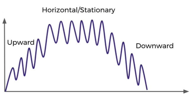
Trends

• Describes on average what is the value doing. A trend tells us what is happening the the mean value e.x. moving upwards (increasing), staying stationary or going downwards (decreasing)

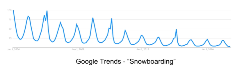
Seasonality

• Seasonality is a repeating trend or pattern, it tells us if there is a repetitive trend. E.x. A general trend can go downwards but have a seasonality that increases every certain months so you can pinpoint a season

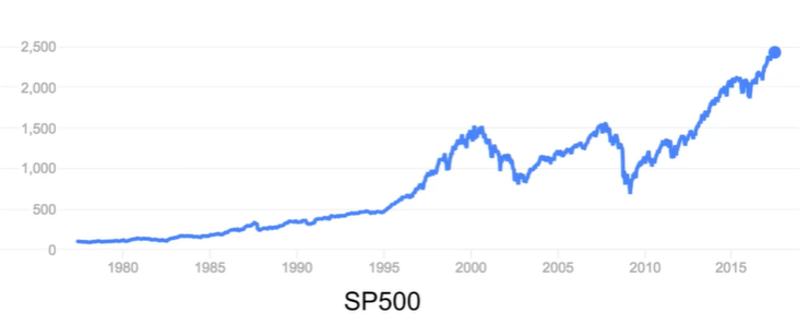
Cyclical

• Refers to trends with no repetition, no seasonality E.x. a stock that sometimes go up sometimes go down but there is no pattern or repetition of trends so you cannot pinpoint a season

statsmodels

• Python library to deal wth Time Series data, allows us to explore data, estimate statistical models and perform statistical testss

• statsmodel comes with datasets that can be used for testing purposes

• Using statsmodels to get the trend of time series can be done with the Hodrick-Prescott Filter that separates a time series $y_t$ into a trend $\tau_t$ and cyclical component (cycle) $\zeta_t$

$$y_t = \tau_t + \zeta_t$$

import os
import seaborn as sns
import numpy as np
import pandas as pd
import matplotlib
matplotlib.use('agg')
import matplotlib.pyplot as plt
import statsmodels.api as sm
import statsmodels.formula.api as smf

base_path = "/home/ubuntu/"

# Load statsmodels data
df = sm.datasets.macrodata.load_pandas().data

# Get Data information
print(sm.datasets.macrodata.NOTE)
print(df.head())

# Generate index with statsmodels and update dataframe index
index = pd.Index(sm.tsa.datetools.dates_from_range(start='1959Q1', end='2009Q3'))
df.index = index
print(df.head())

# Calculate trend
gdp_cycle, gdp_trend = sm.tsa.filters.hpfilter(df["realgdp"])
df["trend"] = gdp_trend

# Plot portion of data and trend
fig = df[["realgdp", "trend"]]["2000-03-31":].plot(figsize=(16, 6)).get_figure()
fig.savefig(os.path.join(base_path, "my_fig.png"))

ETS Models

• ETS (Error-Trend-Seasonality) Models Try to take Error, Trend or Seasonality terms for smoothing purposes and may perform other linear transformations

• A Time Series Decomposition with ETS is method of breaking down a time series into Error/Residual, Trend or Seasonality terms

EWMA Models

• Simple Moving Average weak points:

  • It can gives more noise than signal in a smaller window
  • We will have missing data at the beginning
  • Doesn't really inform about possible future behavior, only describes trend
  • Extreme historical values can really affect the MA

• EWMA (Exponential Waving Moving Average) is an alternative to Moving Average if we want to avoid its weak points since it puts more weight on values that occurred more recently, span can be thought as the time window size. E.x. set to 12 in a time series where each point is data for a month this will mean 12 month EWMA

import os
import seaborn as sns
import numpy as np
import pandas as pd
import matplotlib
matplotlib.use('agg')
import matplotlib.pyplot as plt
import statsmodels.api as sm
from statsmodels.tsa.seasonal import seasonal_decompose

base_path = "/home/ubuntu/"

# EWMA
airline = pd.read_csv(os.path.join(base_path, "airline_passengers.csv"), index_col="Month")
airline.dropna(inplace=True)
airline.index = pd.to_datetime(airline.index)

airline['6M SMA'] = airline['Thousands of Passengers'].rolling(window=6).mean()
airline['12M SMA'] = airline['Thousands of Passengers'].rolling(window=12).mean()
airline['12M EWMA'] = airline['Thousands of Passengers'].ewm(span=12).mean()

airline.plot(figsize=(16, 6)).get_figure().savefig(os.path.join(base_path, "EWMA.png"))

# ETS
result = seasonal_decompose(airline['Thousands of Passengers'], model="multiplicative")
fig = result.plot()
fig.set_size_inches(10, 16)
fig.savefig(os.path.join(base_path, "ETS.png"))

ARIMA Models

• ARIMA (AutoRegressive Integrated Moving Averages) Models is generalization of the ARMA (AutoRegressive Moving Averages) Models, these modesl are used for predict future points in a time series (forecasting). Types:

  • Non-Seasonal ARIMA: for data without repetions or patterns (no season) - we need to set p, d and q
  • Seasonal ARIMA: for data witha repetition pattern or season - we need to set additional P, D and Q

• ARIMA Models are usually not used for financial data because they assume the Y values have a strong connection or correlation to the time ; stocks and financial assets follow a random walk (they go up and down), for those other models like Montecarlo are used

• Components of ARIMA models:

  • AR (p) - Autoregrerssion: Regression model that uses the relationship between the current and previous observations over a period
  • I (d) - Integrated: Differencing of observations (substracts an observation from a previous one)
  • MA (q) - Moving Average: Model that uses the dependency between an observation and a residual error from a MA

• Stationary data

  • Data has a constant mean and variance over a period of time
  • Allows us to predict the mean and variance in a future period of time
  • The average values is constant throughout a period of time
  • Variance should not be a function of time
  • Covariance should not a function of time
  • The Augmented Dickey-Fuller test is a math test toc check for Stationary data

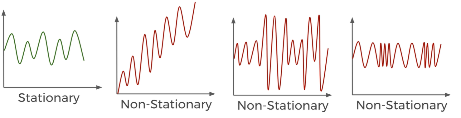
• To use ARIMA we need with stationary data in case our data is not stationary we can transform it through differencing which means just substract previous value $y_t = x_t - x_{t-1}$ where $x$ are the original values and $y$ are the new values, this comes with the cost of losing one value at the beginning of the data set

ACF & PACF

• Autocorrelation plots (Correlogram) shows the correlation of a data sets with itself shifted by $x$ time units, in these plots y-axis is the correlation coefficient and x-axis is the number of units the data was shifted

  • Take the data set $T1$ of length $T$ an make a copy of it to get $T2$
  • Delete first observation of $T1$ (shift left) and delete last observation of $T2$ (shift right)
  • Now you have two series of length $T-1$
  • Calculate correlation coefficient and plot it in $x=1$
  • Repeat this by other values of $x$

• Types of autocorrelation plots:

  • Gradual Decline: Gradually declining as we increase the number of shits
  • Sharp Drop-off: Large positive or negative value at first then it hovers around zero

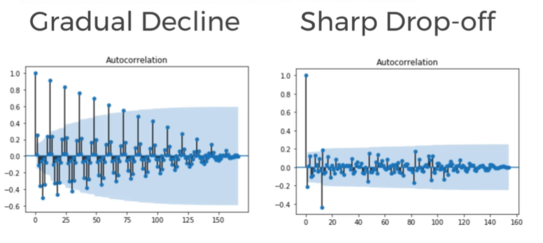
• We use the autocorrelation plots to determine if we will use the AR, MA or both components of an ARIMA model, when we use AR or MA we set the p and q

  • Positive correlation at $x=1$ we use AR <-> Sharp Drop-off
  • Negative correlation at $x=1$ we use MA <-> Gradual Decline

• Partial autocorrelation plots are conditional correlation, it is the correlation between two variables under the assumption that we know and take into account the values of some other set of variables

ARIMA Implementation

• ARIMA general process:
  0. Read Data
  1. Visualize the Time Series Data
  2. Make the time series data stationary
  3. Plot Correlation and Autocorrelation to get which parameters to use in ARIMA
  4. Construct ARIMA Model with previously defined parameters
  5. Use ARIMA to make predictions

import os
import pandas as pd
import matplotlib
import seaborn as sns
import matplotlib.pyplot as plt
import statsmodels.api as sm
from statsmodels.tsa.seasonal import seasonal_decompose
from statsmodels.tsa.stattools import adfuller
from statsmodels.graphics.tsaplots import plot_acf, plot_pacf
from pandas.plotting import autocorrelation_plot
from statsmodels.tsa.arima_model import ARIMA
from pandas.tseries.offsets import DateOffset

base_path = "."

# 0. Read Data
df = pd.read_csv(os.path.join(base_path, "monthly-milk-production-pounds-p.csv"))
df.columns = ["Month", "Milk in Pounds Per Cow"]
df.drop(len(df)-1, axis=0, inplace=True)
df["Month"] = pd.to_datetime(df["Month"])
df.set_index("Month", inplace=True)
print(df.describe().transpose())

# 1. Visualize the Time Series Data
# df.plot()
"""
time_series = df["Milk in Pounds Per Cow"]
time_series.rolling(window=12).mean().plot(label='12 Month Moving Average')
time_series.rolling(window=12).std().plot(label='12 Month STD')
time_series.plot()
plt.legend()
decomp = seasonal_decompose(x=time_series, period=12)
decomp.plot()
"""

# 2. Make the time series data stationary
# 2.1 First check whether data is stationary
# Small p-value (<= 0.05) points to stationary data
# large p-value (> 0.05) points to non-stationary data
def adf_check(time_series):
    result = adfuller(x=time_series)
    print("Augmented Dicky Fuller test for '{}'".format(time_series.name))
    labels = ["ADF Test Stat", "p-value", "# of lags", "Num of Observations used"]
    for value, label in zip(result, labels):
        print("{} : {}".format(label, value))
    if result[1] <= 0.05:
        print("Evidence points to stationary data")
    else:
        print("Evidence points to non-stationary data")
    print("{}".format('-'*20))


df["First Diff"] = df["Milk in Pounds Per Cow"] - df["Milk in Pounds Per Cow"].shift(1)
df["Second Diff"] = df["First Diff"] - df["First Diff"].shift(1)
df["Seasonal Diff"] = df["Milk in Pounds Per Cow"] - df["Milk in Pounds Per Cow"].shift(12)
df["Seasonal First Diff"] = df["First Diff"] - df["First Diff"].shift(12)

# df["First Diff"].plot()
# df["Second Diff"].plot()
# df["Seasonal Diff"].plot()
# df["Seasonal First Diff"].plot()

adf_check(time_series=df["Milk in Pounds Per Cow"])
adf_check(time_series=df["First Diff"].dropna())
adf_check(time_series=df["Second Diff"].dropna())
adf_check(time_series=df["Seasonal Diff"].dropna())
adf_check(time_series=df["Seasonal First Diff"].dropna())

# 3. Plot Correlation and Auto-correlation
# plot with statsmodels
# fig_first = plot_acf(df["First Diff"].dropna())
# fig_sec = plot_acf(df["Seasonal First Diff"].dropna())

# plot with pandas
# autocorrelation_plot(df["First Diff"].dropna())
# autocorrelation_plot(df["Seasonal First Diff"].dropna())

# Positive correlation so we use AR <-> Sharp Drop-off
# plot_acf(df["Seasonal First Diff"].dropna())
# plot_pacf(df["Seasonal First Diff"].dropna())

# 4. Construct ARIMA Model
model = sm.tsa.statespace.SARIMAX(df["Milk in Pounds Per Cow"], order=(0, 1, 0), seasonal_order=(1, 1, 1, 12))
result = model.fit()
print(result.summary())
#result.resid.plot()
#result.resid.plot(kind="kde")

# 5. Make predictions with ARIMA
n_months_ahead = 24
future_dates = [df.index[-1] + DateOffset(months=x) for x in range(1, n_months_ahead)]
future_df = pd.DataFrame(index=future_dates, columns=df.columns)
final_df = pd.concat([df, future_df])

final_df["forecast"] = result.predict(start=len(df), end=(len(df)+n_months_ahead))
final_df[["Milk in Pounds Per Cow", "forecast"]].plot()

plt.show()

References

• Python for Financial Analysis and Algorithmic Trading
• Matplotlib Gallery
• Matplotlib Tutorial by Nicolas P. Rougier & Matplotlib Scipy tutorial
• Order Book & Options Trading
• Statsmodels Time Series Doc & Statsmodels Examples
• EWMA reference
• ARIMA Models reference & p, d, q in ARIMA